Igor Pro Dialogs

This file contains reference material. It is not expected to be read from beginning to end.

Dialog Overview

Most of Igor's dialogs are designed with common features. This topic describes some of those common features.

Operation Dialogs

Menus and dialogs provide easy access to many of Igor's operations.

When you choose a menu item, like Data→Make Waves, Igor presents a dialog:

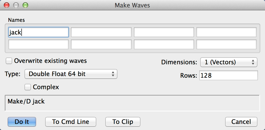
As you click and type in the items in the dialog, Igor generates an appropriate command. The command being generated is displayed in the command box near the bottom of the dialog.

As you get to know Igor, you will find that some commands are easier to invoke from a dialog and others are easier to enter directly in the command line. There are some menus and dialogs that bypass the command line, usually because they perform functions that have no command line equivalents.

Dialog Wave Browser

In dialogs in which a wave must be selected, Igor presents a list of suitable waves in a dialog wave browser. The browser also lets you navigate through the data folder hierarchy.

Double-click a data folder icon to make that data folder the top level for the hierarchical display. To return to levels closer to the root, use the menu at the top of the browser.

In dialogs that support selection of multiple items, you can drag the mouse over items to select more than one. Press Shift while clicking to add additional contiguous items to a selection. Press Ctrl while clicking to add additional discontiguous items to a selection.

You can change the columns that are displayed in the browser by right-clicking the header and enabling or disabling the different columns. If you click on a column in the header area, the waves in the browser are sorted by that column. Click the column in the header area again to reverse the sort direction.

After toggling the display of one or more columns, you may wish to right-click the header again and choose Size All Columns to Fit. You can also resize the columns by dragging the vertical bar that separates columns.

Click the gear icon at the bottom of the browser to display the options menu. It allows you to control whether data folders are displayed and how the waves are sorted and grouped.

To filter waves by name, type a name in the Filter edit box. Only waves whose name match the filter string are displayed. The filtering algorithm supports the following features:


?	Matches any single character.
*	Matches zero or more of any characters. For example, "w*3" matches wave3, wave30 and wave300.
[...]	Matches a single character if it is included in the set of characters specified in square brackets. For example, [A-Z] matches any character from A to Z, case-insensitive. [0-9] matches any single digit.

Click the question mark icon at the bottom right corner of the browser to display a tooltip containing information about the current filter. This tip shows you the filtering criteria currently in place and may help you to figure out why waves you expect to be able to select are not displayed in the browser.

Operation Result Chooser

In most Igor dialogs that perform numeric operations (Analysis menu: Integrate, Smooth, FFT, etc.) there is a group of controls allowing you to choose what to do with the result. Here is what the Result Chooser looks like in the Integrate dialog:

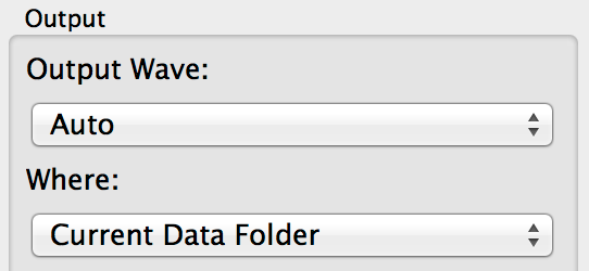
The Output Wave menu offers choices of a wave to receive the result of the operation:


Auto	Igor will create a new wave to receive the results. The source wave is not changed. The new wave will have a name derived from the source wave by adding a suffix that depends on the operation. Selecting Auto makes the Where menu available.
Overwrite Source	The source wave (the wave that contains the input data) will be overwritten with the results of the operation. This will destroy the original data. The Where menu will not be available.
Make New Wave	This is like the Auto choice, but an edit box is presented in which you type a name of your own choosing. Igor will make a new wave with this name to receive the results of the operation. This selection makes the Where menu available.
Select Existing Wave	A Wave Browser will be presented allowing you to choose any existing wave to be overwritten with the results. This choice preserves the contents of the source wave, but destroys the contents of the wave chosen to receive the results.

The Where menu offers choices for the location of a new wave created when you choose Auto or Make New Wave. Usually you will want to choose Current Data Folder.


Current Data Folder	The new wave is created in the current data folder. If you don't know about data folders, this is probably the best choice.
Source Wave Data Folder
	The new wave is created in the same data folder as the source wave. It is quite likely that the source wave will be in the current data folder, in which case this choice is the same as choosing Current Data Folder.
Select Data Folder	This choice presents a Wave Browser in which you can choose a data folder where the new wave will be created.

The Where menu is disabled if you have no data folders other than root. It is also disabled if the Output Wave mode is Overwrite Source or Select Existing Wave.

Operation Result Displayer

In some Igor dialogs that perform numeric operations (Analysis menu: Integrate, Smooth, FFT, etc.) there is a group of controls allowing you to choose how to display the result. Choices are offered to put the result into the top graph, a new graph, the top table, or a new table. For two-dimensional results, New Image and New Contour are also offered. If the result is complex, as is the case for an FFT, New Contour is not available.

Here is what the Result Displayer looks like in the Smooth dialog:

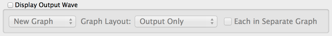
The contents of the displayer are not available here because the Display Output Wave checkbox is not selected. This is the default state.

When you select New Graph, there are four choices in the Graph menu for the contents and layout of the new graph. In this menu, "Src" stands for Source. It is the wave containing the input data. Output is the wave containing the result of the operation.

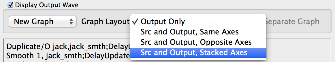
In many cases, the second choice, Src and Output, Same Axes, will not be appropriate because the operation changes the magnitude of data values or the range of the X values.

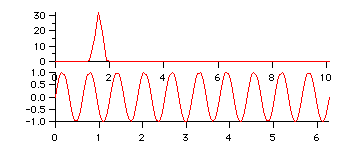
This picture shows the result of an FFT operation when Src and Output, Stacked Axes is chosen:

When you select New Image or New Contour to display matrix results, the Graph Layout menu allows only Output Only or Src and Output, Stacked Axes. The axes aren't really stacked - it makes side-by-side graphs. It makes little sense to put two images or two contours on one set of axes.

The Result Displayer doesn't give you many options for formatting the graph, and doesn't allow any control over trace style, placement of axes, etc. It is intended to be a convenient way to get started with a graph. You can then modify the graph in any way you choose.

If you want a more complex graph, you may need to use the New Graph dialog (select New Graph from the Windows menu) after you have clicked Do It in an operation dialog.

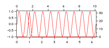
If you select Top Graph instead of New Graph, the output wave will be appended to the top graph. It is assumed that this graph will already contain the source wave, so there is no option to append the source wave to the top graph. The Graph Layout menu disappears, and two menus are presented to let you choose axes for the new wave:

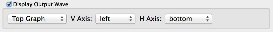
The menus allow you to choose the standard axes- left and right in the V Axis menu, top and bottom in the H Axis menu. If the top graph includes any free axes (axes you defined yourself) they will be listed in the appropriate menu as well.

In most cases the source wave will be plotted on the left and bottom axes. You will usually want to select the right axis because of the differing magnitude of data values that result from most operations. You may also want to select the top axis if the operation (like the FFT) changes the X range as well.

Here is the result of choosing right and top when doing an FFT (this is the same input data as in the graph above):

Note that the format of the graph is poor. We leave it to you to format it as you wish. If you want a stacked graph, it may be better to choose the New Graph option.

Dialog Help

Macro Errors During Experiment Load

For some reason an error occurred while Igor was executing macros that it generated when you last saved the experiment. These macros are used to regenerate the various graphs and other windows that you were using when you saved.

You have the following options:

Click the Quit Macro button. This will stop execution of the current macro (which is probably trying to create a window) but the experiment load will continue. After the load is complete, Igor will create a notebook that provides information about the problem.
Click the Abort Experiment Load button. This aborts the experiment load immediately and displays some diagnostic information.
Fix the macro. If the line of macro code that is in error is drawn inside a box, then you can edit that line and then click the Retry button. Obviously, you need to be somewhat familiar with Igor's macro language to do this. If you have no idea how to fix the line, you might try deleting the entire line and then clicking Retry.

Missing Folder Dialog

Igor displays this dialog during an experiment load if Igor can't find a folder needed to load the experiment. Before displaying this dialog, Igor tries a number of techniques that usually automatically find folders that you have moved or renamed.

If you click the "Skip this Path" button then it is likely you will hit another error later in the experiment load when Igor needs to use this path in order to load another file or group of files.

Skip All Waves From Missing Folder Dialog

Igor displays this dialog if it cannot find the folder referenced by an Igor symbolic path (see Symbolic Paths) during experiment loading. If this occurs, and if the folder is needed to load Igor binary wave files (typically .ibw files), you normally would get a dialog for each missing wave file allowing you to locate the file.

If the folder is really missing, as opposed to merely moved or renamed, then you cannot locate the missing wave files. Clicking Yes in this dialog tells Igor to skip displaying the possibly numerous subsequent missing wave file dialogs.

If you check the Do Not Show This Message Again checkbox, in the future Igor will skip this dialog and instead act like you clicked Yes or No depending on which button you clicked when the checkbox was checked. This is useful for cases where you are rarely or never able to locate missing wave files. The Yes or No response is recorded in Igor's "Igor Pro 10.ini" preference file via the SkipAllWavesFromMissingFolder entry in the DontAskMeDialogs section.

Missing Wave File Dialog

You get this dialog if you share a wave file between experiments and then move, rename or delete the wave file or move the experiment to another computer. If you click the "Skip this Wave" button then you will hit another error or, more likely, a whole set of errors later in the experiment load if Igor needs this wave to recreate a graph or table.

Missing File Dialog

You get this dialog if you open a stand-alone notebook or procedure file and then move, rename or delete the file or move the experiment to another computer. If the file in question is nonessential, there is no harm in skipping it. If it is a procedure file that other procedures depend on, you will get errors when you try to compile or use the missing procedures.

Loading General Text Dialog

This dialog provides wave names for a block of data. If you use the Load Waves dialog (choose Data→Load Waves→Load Waves) and select the "Auto Name & Go" checkbox then this dialog will be skipped.

Save Graphics File Dialog

PDF (Portable Document Format) is Adobe's platform-independent vector graphics format. It is the best format if the destination program supports it.

EPS (Encapsulated PostScript) is a common platform-independent vector graphics format often used by journals. It should be used only if the destination program does not support PDF.

The PNG format is useful for the web and for destination programs that do not support PDF or EPS. PNG is compressed so file sizes are reasonable and PNG tends to be faithfully reproduced by a wide variety of programs. Use 4x or 8x resolution if high resolution is needed.

EMF is the Windows standard for pictures and is generally your first choice if the destination program does not support PDF and if you don't mind using a platform-specific file format.

Choose Text Encoding Dialog

This dialog appears when Igor is unable to open a plain text file because it does not know what text encoding the file uses.

A plain text file is encoded according to some text encoding. The most commonly-used text encodings in Igor are UTF-8 (a byte-oriented form of Unicode), MacRoman, Windows-1252 and Shift JIS.

Igor stores all text internally as UTF-8. When opening a plain text file, it must convert the file's text to UTF-8. This requires that Igor know the file's text encoding, but plain text files usually contain no information indicating what text encoding they use.

Igor uses rules described under Determining the Text Encoding for a Plain Text File to choose the presumed text encoding of the file.

If Igor gets a text encoding error when it tries to convert a file's text to UTF-8 for internal storage, it displays the Choose Text Encoding dialog. You must select the appropriate text encoding for the file and click the Load Using Text Encoding button. If you click Cancel, the file open operation is cancelled.

Handling Text Encoding Errors

By default, Igor treats text encoding errors as fatal. This means that, if Igor is unable to convert text from a given text encoding to UTF-8, you cannot open the file using that text encoding.

In some cases, this is too strict. For example, you may have a file that you know contains Shift JIS (Japanese), but Igor refuses to open it as Shift JIS. This is most likely because the file was written incorrectly or was damaged and contains sequences of bytes that are illegal in Shift JIS. For an example of how this might occur, see Invalid Text Problems.

Although the file is damaged, the bulk of it might be OK. For this case, the Choose Text Encoding dialog allows you to change how text encoding errors are handled. You do this using the Error Handling pop-up menu in the dialog. It offers the following options:

Errors are fatal

Igor refuses to load the file using a given text encoding if the file contains characters that are invalid in that text encoding. You must choose another text encoding or cancel the file open operation.

Replace bad characters with substitute

Igor replaces invalid characters with the Unicode replacement character (�).

This mode allows you to load the file and to see where the errors occurred, by searching for the Unicode replacement characters. You can manually edit the text as desired.

If you save the file without removing the replacement characters, Igor saves the file using the UTF-8 text encoding. Igor 6 does not support UTF-8 so, if you open the file in Igor 6, non-ASCII characters will appear as gibberish.

Skip bad characters

Igor skips invalid characters altogether and loads the valid characters only from the file.

This mode allows you to load the file but you cannot see where the errors occurred.

Replace bad characters with escape codes

Igor replaces invalid bytes with hex escape codes (e.g., \xFE).

This mode, of use mainly for experts, allows you to load the file and to see where the errors occurred, by searching for the hex escape codes. You can manually edit the text as desired.

Handling Null Bytes

Normally plain text files should not contain null bytes (bytes whose value is 0).

In rare cases, you might have a file with null bytes. In those case, you can check the Allow Null Bytes checkbox in order to load the file.

Resolve Text Encoding Conflict Dialog

This dialog appears when you open a procedure file and then add a TextEncoding pragma or change a TextEncoding pragma so that the text encoding specified by the pragma is different from the text encoding used to open the file.

Normally in this case you will want to change the file's text encoding to the text encoding that you specified in the text encoding pragma. To do this, click the Set File to Pragma Text Encoding button. This sets the text encoding that will be used when the procedure file is subsequently saved to disk.

If you inadvertently changed the pragma, click Set Pragma to File Text Encoding. This makes the pragma consistent wiith the text encoding used to open the file.

If you want to manually fix the conflict, click the Cancel Compile button and edit the procedure file.

Export Graphics Dialog

Export Graphics uses the clipboard. Another way to export graphics to another application is to save the graphic in a file. Select Save Graphics from the File menu.

warning

Not all formats are supported by other programs via the clipboard. Support for JPEG and SVG is limited. You will need to experiment.

The selected graphics export format is remembered separately for graphs, page layouts, tables and Gizmo plots. Gizmo supports only bitmap formats.

The selected format is used if you choose Edit→Copy on a graph, page layout or Gizmo plot.

PDF (Portable Document Format) is Adobe's platform-independent vector graphics format. It is the best format if the destination program supports it.

The PNG format is useful for the web and for destination programs that do not support PDF. PNG is compressed so file sizes are reasonable and PNG tends to be faithfully reproduced by a wide variety of programs. Use 4x or 8x resolution if high resolution is needed.

EMF is the Windows standard for pictures and is good for vector graphics if you don't mind using a platform-specific format.

PDF is a good cross-platform choice if the program to which you are exporting supports it.

PNG is a the recommended choice for image plots and Gizmo plots which are inherently bitmaps.

JPEG and SVG are supported by Microsoft Office but not by most other programs.

Substitute Font Dialog

This dialog appears only when a command specifies the name of a font that is not installed on your computer and you have not already specified a replacement font for it.

Use this dialog to choose an installed font to replace the missing one.

You can choose one of:

A replacement for only the current Igor experiment
A replacement for this and all future Igor experiments opened on your computer
No replacement, in which case Igor will generate the usual macro or function error dialog

The command that caused the error is unaltered and still contains the name of the missing font. However, the act of choosing a replacement font prevents another occurence of the Substitute Font dialog from appearing again, because Igor substitutes the replacement font you choose here.

You can edit the substitution at a later time with the Font Substitutions menu item in the Misc menu.

See : Edit Font Substitution Dialog and Font Substitution for a description of how font substitution works.

Edit Font Substitution Dialog

Use this dialog to choose an installed font to replace missing fonts.

You can choose:

A replacement for only the current Igor experiment or
A replacement for this and all future Igor experiments opened on your computer

When a missing font is "replaced", Igor uses the name of the replacement font instead of the font name specified in the command.

The name of the missing font is "replaced" only in the sense that the altered or created object (window, control, etc) uses and remembers only the name of the replacement font.

The command, however, is unaltered and still contains the name of the missing font.

"User" vs "User and Igor" Replacements

Igor employs two levels of font substitution.

The first level is an optional user-level font substitution which overrides the second level. In the dialog only the user-level substitutions are displayed when the pop-up menu is set to "User Replacements":

The second level is Igor's built-in substitution table which substitutes between fonts normally installed on various Macintosh and Windows operating systems. For example, it substitutes "Arial" (a standard Windows font) for "Geneva" (a standard Macintosh font) if Geneva is not installed (which it usually isn't on a Windows computer).

The second-level substitutions are added to the list when the pop-up menu is set to "User and Igor Replacements".

The "Igor Replacements" are hard-coded into Igor's source code, so they can't be altered. That's why the In All Exps checkbox is disabled for Igor Replacements.

Igor Replacements can be overridden with User Replacements, though. When you change the Replacement Font of an Igor Replacement, an overriding User Replacement is created with the same Missing Font. Only the User Replacement is shown in the list.

If you click the Remove Missing Font button, the User Replacement is removed, but the Igor Replacement remains and is shown in the list as it was before the User Replacement was added.

Japanese Igor Replacements

The built-in Igor Replacements include substitutions for Japanese fonts too. By default these aren't shown unless you're using the Japanese-translated version of Igor, but you can show them by selecting User and Igor Replacements and then Show Japanese Replacements from the Replacements pop-up menu.

Default Font Dialog

Default Font selects the default font for text in graphs and page layouts. The default font is used for tick mark labels, axis labels and annotations unless you explicitly select a different font.

When you change the default font, all graph and page layout windows are redrawn using the new font.

Pictures Dialog

This dialog shows all pictures in The Picture Gallery of the current experiment.

Whenever you paste a picture from another program into a page layout or into the drawing layer of a graph, layout or control panel, the picture is given a name is added to the collection.

You can also explicitly add a picture from the clipboard using the Load button in the dialog. Use the popup menu to choose among multiple clipboard types.

The Place Picture button places a picture in the top windows. You can place a picture from the collection into a page layout or drawing layer. You can also place an unnamed copy of a picture into a formatted notebook.

You can rename a picture by clicking the name and entering a new name.

You can delete unused pictures from the collection using the Kill button.

You can convert a picture into the cross-platform PNG format. Converting to PNG may lose resolution and changes vector graphics into bitmaps.

When converting to PNG you can convert in low resolution (screen resolution) or high resolution (8x screen resolution). Converting in high resolution takes a fair amount of space in memory and on disk but provides better looking graphics provided that you are starting from a high-resolution picture. If you are converting a low-resolution picture such as a screen dump then there is no need to use high resolution.

You can copy the selected picture back to the clipboard as either a normal picture or as a text-representation "proc picture" (see Proc Pictures) that can be used in procedures.

Adopt Window Dialog

Adoption is a way for you to copy a procedure or notebook file into the current experiment and break the connection to its original file. The reason for doing this is to make the experiment self-contained so that, if you transfer it to another computer or send it to a colleague, all of the files needed to recreate the experiment will be stored in the experiment itself.

You should save the current experiment after adopting a file.

Adoption does not cause the original file to be deleted. You can delete it on the desktop if you want.

Object Status Dialog

Use this dialog to examine the status and interdependencies of various Igor objects. You can also use it to examine the numeric and string variables you have created in the current experiment.

The dialog displays the properties of one object, called the "Current Object". The name of the current object appears at the top center of the dialog. You can change the current object by choosing an object from the Current Object pop-up menu, or by selecting an object from either of the two dependency lists.

You create a dependency using an assignment statement with the := operator or using the SetFormula operation.

Objects which depend on the current object are listed on the left, and objects which the current object depends on are listed on the right. Items in these lists are object names preceded by a key indicating the type of object:

Key	Object Type
a:	annotation
c:	control
f:	function
s:	string
t:	task (background task)
v:	variable
w:	wave
:=	dependency formula

Dependencies and Recalculation

Igor tracks dependencies between objects. Dependent objects are updated when objects they on which they depend change. To see a list of dependent objects, choose Dependent Objects from the second popup in the top/middle of the dialog. Then click the first popup.

Igor computes the value of a dependent object using a "dependency formula" which includes the names of other objects on which the object depends. A simple example is:

myWave := anotherWave / 10

which updates the wave myWave based on anotherWave. We say that myWave is a dependent object, that "anotherWave / 10" is the dependency formula, and that myWave depends on anotherWave.

Dependency Status

"Update failed" means that the dependency formula used to compute the current object's value failed, probably because one of the objects named in the formula does not exist, or there is a syntax error in the formula. To see a list of broken objects, choose Broken Objects from the second popup in the top/middle of the dialog. Then click the first popup.

Editing a Dependency Formula

You can create a new dependency formula with the New Formula button, delete one using the Delete Formula button, change an existing formula by typing in the Dependency Formula window and clicking the Change Formula button, and undo that change by clicking the Restore Formula button.

Editing the Current Value of an Object

You can edit the current value of some objects, such as global variables, in the window within the dialog.

You can also edit the text of a dependency formula in the dialog. If the formula involves a user function, the formula also depends on the user function, which you will see in the right-hand dependency list.

If the dependency formula uses global variables, whether in a numeric expression, string expression, or as parameters to a function, this causes the formula to also to depend on the global variables. When you change the formula, you will see the global variables show up in the right-hand dependency list.

You can also edit a dependent user function in the dialog.

Editing the Current Value of a Function - Oddities that May Result

If you edit a function and introduce an error and click Change Function, the function compiler will display an error dialog. If you click Quit Compile, the Object Status dialog will come back up, but it will appear as if all the user-defined functions have vanished. They have not vanished; Igor just can't display information about functions unless all the procedure windows compile successfully. When you fix the error, the user-defined functions will return.

For this reason, it really makes more sense for you to click the Edit Procedure button in the error dialog. This brings up the procedure window in which the function is defined, but it does exit the Object Status dialog first (it would be devoid of function information, anyway). Fix the error, and then reselect the Object Status dialog. You will find that the function is still the current object, and that all is well.

Rename Objects Dialog

Use this dialog to rename waves, variables, strings, symbolic paths, and pictures.

To rename windows use the Control item in the Windows menu.

Use the arrow button to transfer selected items to the list on the right side of the dialog. Edit the name of an item in the edit box under the New Name label.

Double-click to transfer a single item from the browser to the rename list.

Click on a row in the rename list and press Delete or Backspace to remove it from the list.

Make Waves Dialog

Use this dialog to create new waves with specified dimensions, size, data type and names.

You can also create waves by:

Entering numbers or text in a table
Loading data or text from a file
Cloning an existing wave using the Duplicate Waves dialog

See Object Names for rules for naming waves.

After using the Make operation, you should use the SetScale operation to set the scaling for each dimension of the wave, as well as setting the units for each dimension and the data values. The Change Wave Scaling dialog provides a convenient interface to the SetScale operation.

Kill Waves Dialog

When you kill a wave that you no longer need, you free up memory occupied by the wave and also reduce clutter in dialog lists and pop-up menus.

The Kill All Waves Not In Use checkbox applies only to waves in the current data folder. If the current data folder is visible in the dialog's Wave Browser, the data folder icon is marked with a small red arrow.

Delete Source Files applies only to waves that were loaded from, and are still linked to, Igor binary wave files (.bwav or .ibw).

To kill global numeric and global string variables, you must execute the KillVariables or KillStrings commands or use the Data Browser. There are no dialogs for this.

Duplicate Waves Dialog

Duplicating a wave is identical to making a wave except that the new wave has the same dimensionality, number of data points, data type, scaling and contents as the wave which you duplicated. You can use the Range control to specify that you want to duplicate a subrange of the template wave.

Duplicating a wave is often the first step in an analysis task. Many Igor operations, (e.g., Integrate, Differentiate, Smooth) take a wave as a parameter and modify it in place. If you want to preserve your original data, you can use the Duplicate operation to make a clone and then operate on the clone.

Change Wave Scaling Dialog

You use the Change Wave Scaling dialog to set the scaling and units for each dimension, data units and, infrequently, data min/max. It generates SetScale commands.

If your 1D data is evenly spaced, you should use SetScale commands to specify the scaling of the X dimension. We call this "waveform data". For background information on waveform data, see The Waveform Model of Data.

If your 1D data is not evenly spaced, you should not use SetScale but leave the dimension scaling as the default, "point scaling". We call this XY data. For background information on XY data, see The XY Model of Data.

Higher dimensional waves can also be evenly spaced or unevenly spaced. For example, if your data is 2D and is evenly spaced, use SetScale commands to specify X and Y scaling.

For a 1D waveform, Igor stores two X scaling properties, x0 and Δx. It calculates the X values of the waveform using the formula

X = x0 + Δx*P

where P is a zero-based point number.

While there is only one way of calculating X values, there are three ways you can specify the x0 and Δx values. The simplest way is to simply specify x0 and Δx directly. This is the "Start and Delta" mode in the dialog and is the only way of setting the scaling unless you click the More Options button. As an example, if you have data that was acquired by a digitizer that was set to sample at 1 MHz starting 150 µs after t=0, you would enter 150E-6 for Start and 1E-6 for Delta.

The other two ways of specifying X scaling are to tell Igor what the starting and ending X values are and allow Igor to calculate Δx from the number of points. In the "Start and End" mode you specify the X value of the last data point. Using the "Start and Right" mode you specify the X at the end of the last interval. For example, assuming our digitizer (above) created a 100 point wave, we would enter 150E-6 as Start for either mode. If we selected the "Start and End" mode we would enter 249E-6 for End (150E-6 + 99*1E-6). If we selected "Start and Right" we would enter 250E-6 for Right.

What it all boils down to is this:

Use "Start and Delta" mode whenever you know the starting dimension value and delta.
Use the "Start and End" mode when you have a measured dimension value for the last data point.
Use the "Start and Right" mode all other times.

Remember that, regardless of which way you specify dimension scaling, Igor translates this into Start and Delta. If you find the three ways of specifying X scaling confusing, stick to the Start and Delta mode.

In the case of 1D data, P is used for point number, and X for the point position. These are the equivalent terms for other dimensions:


Dimension number:	0	1	2	3
Dimension name:	row	column	layer	chunk
Dimension index:	p	q	r	s
Scaled dimension index:	x	y	z	t

and	X = x0 + Δx*p
		Y = y0 + Δy*q
		Z = z0 + Δz*r
		T = t0 + Δt*s

Units

Enter the units of your data in the Units box. Igor automatically scales your data and inserts SI multiplier prefix symbols (µ,m,k,M, etc.) when it uses your units to create axis labels. Thus if your data is in volts, and with values on the order of 1E-6, set the units to "V". Then the axis label will automatically appear as "µV".

You can use as many characters as you wish in the Units box. Clearly, however, there are many compound units you might enter there that will not work with the automatic prefix feature. We recommend that you use SI units if they apply ("s" for seconds, "V" for volts, etc.), and leave the Units box empty if the units don't work well with the standard prefixes.

Set Data Properties

If your data has an inherent full scale, you can set this with the min and max values. Later you can access these values in the Axis Range tab of the Modify Axis dialog to quickly set axes in graphs based on the wave's min and max. These values are not used to scale the data - they just serve as documentation of the conditions under which the data was taken.

note

You can easily copy scaling from one wave to one or more waves by selecting a wave and reading in the scaling information using the From Wave button. Then select the waves that you want to have the same properties and click Do It. To do the same thing in a procedure, use the CopyScales operation.

Redimension Waves Dialog

Use the Redimension Waves dialog to change the precision, type, number of points, and number of dimensions of one or more waves. When the conversion is done, your data is preserved to the extent possible. However, if you convert a wave from a higher numeric precision to a lower one, you will permanently lose precision.

If you increase the size of a dimension (add points to a 1D wave, or add rows or columns to a 2D wave), Igor appends the additional points to the end of the appropriate dimension with an initial value of 0. If you decrease the size of a dimension, Igor permanently removes points from the end the dimension.

If you change dimensionality of a wave, new dimensions are added filled with zeroes. If you shorten one dimension while creating a new one, the data from the shortened dimension is lost, and the new dimension is filled with zeroes.

As a special case, if converting to or from a 1D wave, Redimension will leave the data in place while changing the dimensionality of the wave. For example, you can use Redimension to convert a 36-element 1D wave into a 6x6 matrix in which the elements in the first column (column 0) are the first 6 elements of the 1D wave, the elements of the second column are the next 6, and so on:

Make/O/N=(36) thirtySixValues
thirtySixValues = p                 // 0 to 35
Redimension/N=(6,6) thirtySixValues
Print thirtySixValues[5][5]         // Prints 35

When redimensioning from a 1D wave, columns are filled first, then layers, followed by chunks.

Insert Points Dialog

The Insert Points dialog generates InsertPoints commands which insert zeroed data values in front of the specified first point. If the first point is greater than the value of the last point then the values are appended to the end of the wave.

You can insert rows or columns into a matrix wave. The new row or column is inserted before the row or column specified by the First Point. Likewise, you can insert rows, columns, or layers into a 3D wave and rows, columns, layers or chunks into a 4D wave.

Inserting points into a 2D wave inserts an entire row or column of zeroes, inserting into a 3D wave inserts the appropriate planar array of zeroes, and inserting into a 4D wave inserts the appropriate volume of zeroes.

Inserting new columns into a 1D wave converts it into a 2D wave. Inserting layers into a 2D wave makes it 3D, and inserting chunks into a 3D wave makes it 4D.

Delete Points Dialog

The Delete Points dialog generates DeletePoints commands which remove data points from the selected waves starting at the specified first Point. You can enter a large value in the Number of Points box to delete all the way to the end of the wave.

Deleting points from a 2D wave deletes an entire row or column, deleting from a 3D wave deletes the appropriate planar array, and deleting from a 4D wave deletes the appropriate volume.

Deleting all but one column of a 2D wave makes it into a 1D wave, deleting all but one layer of a 3D wave makes it 2D, and deleting all but one chunk of a 4D wave makes it 3D.

New Graph Dialog

The New Graph dialog generates Display commands to display waveforms or XY pairs. You typically use it to display 1D waves but the dialog can also generate commands to display parts of multi-dimensional waves, such as columns from 2D waves, as described under Subrange Display.

The dialog has two modes: simple and advanced. You choose the mode using the More Choices or Fewer Choices button.

In the simple mode, you are limited to choosing 1D waves. You can choose multiple Y waves and 0 or 1 X wave. To display waveform data, choose _calculated_ from the X Wave list. To display XY pairs, choose the X wave. Using the Axis popup menus, you can choose the axis against which the waves are to be displayed or create new axes.

The advanced mode allows you to generate far more complex commands that can display 1D waves, subsets of 1D waves, or elements of multi-dimensional waves. It also allows you to generate multiple Display commands by selecting items in the Y Waves and X Wave lists and clicking the Add button. This allows you, for example, to create a graph containing multiple XY pairs where each Y wave has a separate X wave.

To display subsets of 1D waves or elements of multi-dimensional waves, make your selections, click the Add button, and edit the range in the main list. If you enter a single number in an edit cell, it selects that particular row or column for display. Leaving a cell blank indicates that the entire dimension should be used. Enter a range of elements with numbers separated by commas: 10,20 will select eleven elements for display.

Igor initializes the edit cells in the trace list with values for the full range of rows of a wave. If you use a matrix wave, it preselects column zero. If you have X and Y waves of unequal length, the ranges are preset to the lesser of the full number of X or Y rows.

If you want your Y values to run horizontally and your X values to run vertically, you can visit the Modify Graph dialog after you have created the graph to swap the X and Y axes.

You can swap the X and Y axes on a trace-by-trace basis using the Swap Trace X & Y Axes checkbox. Note that this checkbox applies to all traces created during a single visit to the dialog.

The standard axes, left, right, bottom, and top, are always fixed to the corresponding edges of the plot area. If you want axes to be in the center or if you want several axes on one side, you can create "free" axes using the New entry in the Axis pop-up menus. Once the graph is generated you can drag free axes anywhere you like (in the direction perpendicular to the axis).

Generally, you do not need to set the title of the graph window. The default title contains useful information about graph contents.

Style macros provide a way to apply predefined styles to new graphs. You must first define your style macro. You can then apply it by choosing its name from the Style popup menu. See Graph Style Macros for details.

See also: Graphs, Display, Subrange Display

Remove from Graph Dialog

The Remove from Graph dialog removes traces, image plots and contour plots from the graph.

Select the type of object you want to remove from the pop-up menu at the top. Removing all the contour traces from a contour plot is not the same as removing a contour plot.

When you remove the last item plotted on a given axis, the axis is removed too.

Modify Graph Dialog

The Modify Graph dialog allows you to change overall graph properties.

The margin settings allow you to specify the distance from the outside edge of the graph to the corresponding axis. The main use for this is to force the left margin of several graphs to be identical so that they look good when stacked vertically in a page layout.

The width and height settings allow you to control the width of horizontal axes and the height of vertical axes using one of five modes. In general, you should leave the modes set to Auto. If you try one of the more exotic modes and find yourself with an unreasonable graph size, set the graph to a reasonable size using the Absolute mode and then switch back to Auto.

If you leave the Graph Font set to Auto then the default font for the graph will be the same as that specified in the Default Font dialog as found in the Misc menu.

New Box Plot Dialog

The New Box Plot Dialog creates box plots.

To change colors, marker types, etc., use the Modify Box Plot Dialog. Choose Graph→Modify Box Plot. The Modify Box Plot Dialog is also available by right-clicking on the box plot trace and selecting Modify Box Plot Appearance.

The New Box Plot Dialog generates a Display command to create a blank graph window, and an AppendBoxPlot command to create the box plot trace. If you select multiple 1D waves as the data for the boxes, it will also generate one or more AddWavesToBoxPlot commands.

Select waves containing the data for your box plot in the list on the left. By default, that list shows 1D waves, and you would select one wave for each box you wish to show in your box plot trace. If your data sets are organized as columns in a matrix wave, select One Multicolumn Wave from the menu above the list.

When you have made your selections, click the arrow button to transfer your selection to the list on the right. If you have selected multiple 1D waves, you can re-order the list on the right. The boxes in the box plot trace will have the order shown in the list on the right.

Box plots may have either a numeric or a category X axis. A numeric X axis will result if you select _calculated_ from the X Wave menu below the right-hand list, or if you select a numeric wave from that menu. A category X axis will result if you select a text wave from the X Wave menu, or if you select _labels_.

The X Wave menu shows only 1D waves with the same number of elements as the number of columns in a selected matrix wave, or the number of 1D waves selected.

Append Box Plot Dialog

The Append Box Plot Dialog adds a box plot trace to an existing graph window. It works just like the New Box Plot Dialog, except that it does not generate a Display command.

Modify Box Plot Dialog

The Modify Box Plot Dialog allows you to alter the appearance of a box plot trace. Select the box plot trace from the list on the left. If you wish to alter the appearance of individual boxes within a box plot trace, you can click the disclosure control at the left end of the box plot trace list entry, and then select individual boxes to alter.

New Violin Plot Dialog

The New Violin Plot dialog creates violin plots.

To change colors, marker types, etc., use the Modify Violin Plot Dialog. Choose Graph→Modify Violin Plot. The Modify Violin Plot Dialog is also available by right-clicking on the violin plot trace and selecting Modify Violin Plot Appearance.

The New Violin Plot Dialog generates a Display command to create a blank graph window, and an AppendViolinPlot command to create the violin plot trace. If you select multiple 1D waves as the data for the violin plot, it will also generate one or more AddWavesToViolinPlot commands.

Select waves containing the data for your violin plot in the list on the left. By default, that list shows 1D waves, and you would select one wave for each data set you wish to show in your violin plot trace. If your data sets are organized as columns in a matrix wave, select One Multicolumn Wave from the menu above the list.

When you have made your selections, click the arrow button to transfer your selection to the list on the right. If you have selected multiple 1D waves, you can re-order the list on the right. The data sets in the violin plot trace will have the order shown in the list on the right.

Violin plots may have either a numeric or a category X axis. A numeric X axis will result if you select _calculated_ from the X Wave menu below the right-hand list, or if you select a numeric wave from that menu. A category X axis will result if you select a text wave from the X Wave menu, or if you select _labels_.

The X Wave menu shows only 1D waves with the same number of elements as the number of columns in a selected matrix wave, or the number of 1D waves selected.

Append Violin Plot Dialog

The Append Violin Plot Dialog adds a violin plot trace to an existing graph window. It works just like the New Violin Plot Dialog, except that it does not generate a Display command.

Modify Violin Plot Dialog

The Modify Violin Plot Dialog allows you to alter the appearance of a violin plot trace. Select the violin plot trace from the list on the left. If you wish to alter the appearance of individual data sets within a violin plot trace, you can click the disclosure control at the left end of the violin plot trace list entry, and then select individual data sets to alter.

New Category Plot Dialog

The New Category Plot dialog creates category plots. A category plot displays one or more numeric Y waves against a set of categories represented by a text wave or by the dimension labels of the first Y wave.

Only 1D waves appear in the Y Waves list. Only text waves and the special keyword "_labels_" appear in the X Wave list. Choose _labels_ to use dimension labels from the first trace as the category labels.

To make a category plot with the categories on the vertical axis and horizontal bars, visit the Modify Graph Dialog (choose Graph→Modify Graph) after creating the category plot and click the Swap X and Y Axes checkbox.

The gaps between bars and categories are set in the Modify Axis Dialog.

Generally, you do not need to set the title of the graph window. The default title contains useful information about graph contents.

Append Category Traces Dialog

The Append Category Traces dialog is much like the New Category Plot Dialog.

You can append traces to existing axes or you can create new axes as part of the append. A category axis can have only one text wave associated with it; if you select an X axis already in use as a category axis (usually the bottom or top axis) you cannot select an X wave.

New Contour Plot Dialog

The New Contour Plot dialog makes a new contour plot. It generates two commands - a Display command to make a blank graph window, and an AppendMatrixContour or AppendXYZContour command to append a contour plot to that graph window.

A contour plot can be created from a matrix wave, a 3 column 2D wave representing X, Y and Z values, or from three 1D waves representing X, Y and Z. You start by choosing the format of your data from the Contour Data popup menu. That controls what waves appear in the lists below.

Select "Matrix of Z Values" to make a contour plot using Z data from a 2D matrix wave. If your matrix data is evenly spaced in the X dimension, select _calculated_ from the X Wave list. If it is evenly spaced in the Y dimension, select _calculated_ from the Y Wave list. If either dimension is unevenly spaced and you have an appropriate X or Y wave, select that wave from the X Wave or Y Wave list. For an NxM data wave, the X wave must have N elements and the Y wave must have M elements.

Select "Matrix of X, Y, Z Columns" to make a contour plot from XYZ triplets stored in a 3 column matrix wave.

Select "X, Y, and Z Waves" to make a contour plot from XYZ triplets stored in three one-dimensional waves.

If you want your Y values to run horizontally and your X values to run vertically, you can visit the Modify Graph dialog after you have created the graph to swap the X and Y axes.

The Appearance button sets characteristics of the contour plot prior to making the plot, using the Modify Contour Appearance Dialog.

Append Contour Plot Dialog

The Append Contour Plot dialog works much like the New Contour Plot Dialog.

You can append a contour plot to existing axes or you can create new axes as part of the append.

Modify Contour Appearance Dialog

You reach the Modify Contour Appearance dialog by choosing Graph→Modify Contour Appearance, by right-clicking a contour plot and choosing Modify Contour, or by pressing Shift while double-clicking inside a contour plot.

Use the dialog to alter various aspects of the contour plot, including number of contour levels, line colors, labeling styles, and label and contour updating.

Updating a contour plot or the labels for a contour plot can be time-consuming, so several levels of updating are provided. You can control when contours are updated using the Update Contours pop-up menu. You can control when labels are updated using the Update Labels pop-up menu. Turning off or restricting updating can result in a graph that doesn't reflect the current state of the data.

Special effects such as dashed contours, special colors for ranges of contour values, or variable line thickness can be achieved by modifying individual contour traces. You can do this by right-clicking a contour trace and using the resulting pop-up menu or by choosing Graph→Modify Trace Appearance.

The Contour Line Colors button brings up a subdialog allowing you to select various built-in color tables, color table waves, color index waves, or a single color for all contour lines.

A nice-looking background for a contour plot is an image display of the same data set. Choose Graph→Append to Graph→Image Plot to add an image plot.

More Contour Levels Dialog

The More Contour Levels dialog appears when you click the More Contour Levels checkbox in the Modify Contour Appearance Dialog.

Any numbers entered in this dialog add contour lines to the contour plot, in addition to the automatic levels, levels specified with a wave, or manual levels.

Contour Line Colors Dialog

The Line Colors dialog appears when you click the Line Colors button in the Modify Contour Appearance Dialog.

The radio buttons on the lefthand side of the dialog allow you to choose a coloring method for the contour lines in your contour plot.

The simplest method is to select Color Table, choose a built-in color table from the pop-up menu, and leave the Auto radio buttons selected. When you do this, Igor maps the full range of contour level values to the full range of the selected color table.

For greater control you can select Color Table Wave or Color Index Wave. See The Color of Contour Traces for details.

See also:

The Color of Contour Traces

Color Table Details

Color Table Waves

Indexed Color Details

Contour Labels Dialog

The Contour Labels dialog appears when you click the Label Tweaks button in the Modify Contour Appearance Dialog. Select label coloring, number format, font, font size, and label rotation from this dialog.

You can choose the rotation of contour labels from tangent, horizontal, vertical or both orientations. If both vertical and horizontal labels are permitted, Igor will choose horizontal or vertical with a preferend for horizontal labels. Selecting one of the Tangent choices creates labels that are rotated to follow the contour line. The "Snap to" alternatives convert labels within 2 degrees of horizontal or vertical to exactly horizontal or vertical.

Igor will try to put the contour labels in "good" places.

If you select "0 and 90" for the Rotation, Igor will select a horizontal or vertical label for a contour depending on the contour's shape. Horizontal labels are preferred.

You can tell Igor that you want only horizontal or vertical labels by selecting 0 or 90 from the Rotation pop-up menu.

You can alter the labels after Igor has made them by double-clicking a contour label and changing it in the resulting Modify Annotation dialog.

You can change the position of a contour label by pressing Alt and dragging the label to a new point on the contour. If you drag a label to a different contour, the label will change to reflect the new value.

Altering an individual label with the Modify Annotation Dialog will prevent Igor from updating the label.

New Image Plot Dialog

The New Image Plot dialog makes a new image plot using intensity values stored as the Z values in a 2D matrix wave, or a true color image using a 3D RGB or RGBA wave.

The dialog normally generates two commands - a Display command to make a blank graph window, and an AppendImage command to append a image plot to that graph window. Selecting the Use NewImage command checkbox replaces Display and AppendImage with the NewImage operation which changes what options you have for creating an image plot in this dialog - see the Use NewImage Command section below for details.

By selecting 1D waves in the X and Y lists you can specify uneven pixel spacing. The X and Y values are the positions of the pixel boundaries, not the pixel centers. Consequently, for an NxM image, the X wave must have N+1 elements and the Y wave must have M+1 elements.

A standard image is displayed upside-down because the usual origin for images is in the top left corner - see Image Orientation for an example. You can display your image rightside up by visiting the Axis Range tab (double-click on the tick labels on the vertical axis) and selecting the Reverse Axis checkbox. Or check the Use NewImage Command checkbox - NewImage automatically reverses the left axes.

If you want your Y values to run horizontally and your X values to run vertically, you can visit the Modify Graph dialog after you have created the graph to swap the X and Y axes.

The Appearance button sets characteristics of the image display prior to making the plot, using the Modify Image Appearance Dialog.

X, Y, and Z Wave Lists

The X Wave, Y Wave, and Z Wave lists show the available waves that will be accepted by the AppendImage operation.

You should select the matrix wave containing your image data in the Z Wave list. This will update the X Wave and Y Wave lists to show only those waves, if any, that may be used with the selected Z wave.

Choosing _calculated_ from the X Wave list uses the row scaling (X scaling) of the matrix selected in the Z Wave list to provide the X coordinates of the image rectangle centers.

Choosing _calculated_ from the Y Wave list uses the column scaling (Y scaling) of the matrix to provide Y coordinates of the image rectangle centers.

You can also select a 1D wave to provide the X or Y values for a matrix of Z values. Only those waves with the proper length for the selected Z Wave are shown in the X Wave and Y Wave lists. See Image X and Y Coordinates for details.

Use NewImage Command

The NewImage command nicely sets the window margins and axes to maximize the image in the window, presets the window size to match the number of pixels in the image, and automatically reverses the left (vertical) axes so that pictures aren't displayed upside down.

However NewImage does not support window titles, 1D X and Y waves, axes other than left and top, or graph style macros.

A useful option of NewImage is the "Do not treat multi-layer images as direct color" checkbox. Selecting that option displays one layer from a three-layer or four-layer 3D wave as a false-color or indexed-color image (the data values in one layer are linearly mapped onto a color table), instead of using all three or four layers to display a direct color image (see Direct Color Details). Click the Appearance button to choose which layer is displayed

Clicking the Appearance button displays the Modify Image Appearance subdialog. The subdialog allows you to specify color properties and how autoscaling is done for multi-layer Z waves.

See also: Image Plots, Display, NewImage, AppendImage

Append Image Plot Dialog

The Append Image Plot dialog works much like the New Image Plot Dialog.

You can append an image plot to existing axes or you can create new axes as part of the append.

Reorder Images Dialog

See: Getting Help

The Reorder Images dialog generates ReorderImages commands which changes the drawing order of images in a graph. The first image in the list is drawn first, which means all other images will draw over it. Use this dialog to alter which images obscure which.

Starting in Igor Pro 10, two layers are available for image graphs. There is Layer 0 which is under any traces and axes in the graph. Layer 0 was previously the only layer available for images. There is now also Layer 1 which is above any traces and axes in the graph. Images may not be inserted between traces or axes, only below all traces and axes and above all traces and axes.

Modify Image Appearance Dialog

The Modify Image Appearance dialog is displayed when you select Graph→Modify Image Appearance or right-click an image and choose Modify Image Appearance from the resulting pop-up menu.

Use the dialog to alter the coloring of a false-color image.

The radio buttons on the lefthand side of the dialog allow you to choose a coloring method for the image plot.

The simplest method is to select Color Table, choose a built-in color table from the pop-up menu, and leave the Auto radio buttons selected. When you do this, Igor maps the full range of image Z values to the full range of the selected color table.

For greater control you can select Color Table Wave, Color Index Wave, or Explicit Mode. See Modifying an Image Plot, Color Table Waves, and Indexed Color Details for details.

The Color Table and Color Table Wave modes give you the option of choosing a "lookup wave". This is rarely used and "_none_" is the usual choice. See Color Table Ranges - Lookup Table (Gamma) for a reason to use a lookup wave.

Explicit Mode specifies a particular color to use with a particular Z value in the image. This is intended for use with integer values. If you use floating-point waves, you may not get the result you expect.

You can remove an Explicit Mode value by selecting the appropriate line in the list and pressing the Backspace or Delete button.

If you make an image using a three-layer wave containing direct RGB values, you cannot alter it with this dialog, unless it has multiple chunks, in which case you can modify only the displayed chunk.

See also:

Modifying an Image Plot

Color Table Details

Color Table Waves

Indexed Color Details

Append Traces Dialog

The Append Traces dialog works much like the New Graph Dialog.

You can append traces to existing axes or you can create new axes as part of the append.

Reorder Traces Dialog

The Reorder Traces dialog generates ReorderTraces command which change the drawing order of traces in your graph. This in turn affects stacking if you are using a stacking drawing mode.

The first trace in the list is drawn first, which means all other traces will draw over it.

To change the order, click one of the items in the list and drag it up or down, above or below another list item.

Use this dialog to alter which traces obscure which. For instance, if you select Fill to Zero for several traces, you will generally want the traces highest in the graph at the back so that the fills overlap correctly.

The trace order is also important in the operation of grouping modes for trace display (see Grouping, Stacking and Adding Modes). These modes allow you to fill between one trace and the next, add a trace to the next, stack bars, and much more.

Modify Trace Appearance Dialog

You reach the Modify Trace Appearance dialog by choosing Graph→Modify Trace Appearance, by right-clicking a trace and choosing Modify <Trace Name>, or by double-clicking a trace in the graph. You can also perform some of the modifications by right-clicking a trace in the graph to get a pop-up menu.

The color of a trace, the size and style of its markers, and the pattern used to fill it if it is displayed as a bar, can each be controlled on a point-by-point basis using another wave to supply the per point setting. To set one or more of these properties based on another wave, click the "Set as f(z)" button. See Setting Trace Properties from an Auxiliary (Z) Wave for details.

The Grouping modes interact with the Mode setting - see Grouping, Stacking and Adding Modes. The trace order is also important in the operation of grouping modes for trace display - see Reorder Traces Dialog.

Contour Plots

Usually the color of traces belonging to a contour plot are set using the Modify Contour Appearance Dialog, but you can override those settings with this Modify Trace Appearance dialog. See Overriding the Color of Contour Traces.

See also:

Modifying Traces

Stacked Bar Charts, Category Plot Pitfalls

The Color of Contour Traces

Setting Trace Properties from an Auxiliary (Z) Wave

Grouping, Stacking and Adding Modes

ModifyGraph

Trace Offset Dialog

Trace offset is for display purposes only, it does not affect the actual data. It is useful for spreading a family of traces apart or aligning two traces so that they can be compared.

You can set the offset independently for X and Y. The regular offset is additive and appropriate for traces plotted against linear axes. The multiplier offset is multiplicative and appropriate for traces plotted against log axes.

You can also set a trace's offsets by clicking it in the graph and holding until the XY offset readout appears in the lower/left corner of the graph. While holding the mouse button down, drag the point you clicked wherever you want it. The rest of the trace will follow along.

When offsetting a trace that uses log axes, the shape of the trace is not changed - it is simply moved. If you were to try to offset a trace by adding a constant to the wave's data, it would distort the trace.

Replace Wave Dialog

The Replace Wave dialog replaces a wave displayed in a graph with another wave.

You can also replace a subrange of a wave with a different subrange of that wave or of another wave.

If you check Replace All in Data Folder, all of the waves in the graph are replaced by the corresponding waves in the specified data folder. The correspondence is based on the wave names.

Modify Axis Dialog

The Modify Axis dialog provides control over graph axes. Most of the settings in this dialog are implemented using the ModifyGraph operation.

There are a number of ways to reach the Modify Axis dialog. Choosing Graph→Modify Axis or double-clicking an axis displays the tab you were last using. Choosing Graph→Set Axis Range or double-clicking tick mark labels brings up the dialog with the Axis Range tab displayed. Choosing Graph→Label Axis item or double-clicking an axis label brings up the dialog with the Axis Label tab displayed.

You can apply changes to a single axis or to multiple axes using the Axis popup menu.

Checking the Live Update checkbox causes your graph to be redrawn every time you change a setting in the dialog. This can be very helpful, but very annoying if the graph takes a long time to redraw.

Axis Tab

When a log axis is selected, the LogLin checkbox is made available. Selecting LogLin forces Igor to use a linear tick value (or exponent value) method when the range of the axis is small or large. See Log Axes.

Igor draws a Date/Time axis if the units of the controlling wave are "dat". The Date/Time mode selection is a shortcut to change the units for the appropriate wave. The change is made as soon as you select the radio button. The old units are remembered and are restored if you click the Cancel button or if you select linear or log mode.

The Mirror Axis pop-up menu contains Off, On, No ticks and Labels items. If you turn Mirror Axis on for the left or bottom axis then the right or top axis will be a mirror image of the opposite axis. A mirror axis that is on has tick marks but no tick labels. In the no ticks state the mirror axis has no tick marks. In the labels state, the mirror axis has tick marks and tick labels. If you previously appended a wave to the graph and you specified Use Right Hand Axis or Use Top Axis then you cannot turn Mirror Axis on for that axis.

There are two ways in Igor to control the spacing between the edge of the graph and the edge of the plot area (the rectangle in which traces are plotted). The Axis Offset item in this dialog tweaks the position of each of the four standard axes (left, right, bottom and top) which in turn define the plot area. The position of the axis is still variable depending on font size, tick label lengths, etc. On the other hand, the Axis Margin items found in the Modify Graph dialog set the absolute distance between the edges of the graph and the edges of the plot rectangle. This freezes the axis position.

In general, if your graph will be standing alone and you are unsatisfied with the axis position then you should simply drag the axis as desired. That effectively sets the Axis Offset item in this dialog interactively. On the other hand if your graph will be used with others in a page layout and you want the axes from all the graphs to line up (i.e., stacked graphs) then you should use the Axis Margin setting in the Modify Graph dialog to set equal numerical values for all the graphs. Note that the Axis Margin setting in the Modify Graph dialog overrides the Axis Offset setting in this dialog. An easy way to set all graph margins to be uniform in a layout is via the Make Plot Areas Uniform selection from the Layout menu.

Normally Igor offsets axes so that waves do not cover them. The Axis Standoff checkbox disables this behavior. If you disable axis standoff, part of the wave may cover the axis. This is especially noticeable when you use markers and autoscale the graph.

note

Axis Standoff is ignored if a standard axis has been set to have a reduced extent, that is, if the Draw Between settings in this dialog are not 0 and 100%. This is to simplify the creation of graphs with stacked axes.

Error Bars Dialog

Choose the source of error information from the Y Error Bars and X Error Bars pop-up menus.

If you want single-sided error bars or bars that have different directions at different data points or if you want to suppress bars at certain locations then you will need to use the "+/- wave" mode.

You can get single-sided error bars by providing just one error wave and can change the direction of individual bars by simply changing the sign of individual error values. You can eliminate individual bars by setting their error values to NaN (missing value).

In "+/- wave" mode, only waves having at least as many points as the trace are shown in the pop-up wave browsers. If you select a wave with more points, or a multidimensional wave, you must specify a subrange using the Subrange button.

Click Use Shading Instead of Bars to indicate errors using shading. By default, the shading foreground color is black with an alpha of 0. In this case, Igor uses the trace color with an alpha of about 0.3 making the shading translucent. You can change the color and transparency of the shading using the Foreground Color pop-up menu.

Set as f(z) Dialog

Various aspects of the trace display can be controlled on a point-by-point basis by another wave (a "Z wave").

If you select a Z wave with more points than the wave controlling the trace you are modifying, you need to select a subrange of the Z wave using the Subrange button.

Color as f(z)

If Color Mode is set to Color Table, select a Z wave to control the color of the trace display. Igor sets the colors by mapping the data range in the Z wave to the range of colors in the selected color table. Z values that fall outside of the range can be drawn with selected colors, be drawn transparent (missing), or be drawn with the closest color from the color table (which is the default). See Color Tables for details.

The remaining Color Modes use 3 column RGB or 4 column RGBA waves. Only waves that have exactly three or four columns are shown in the pop-up menu.

If Color Mode is set to Color Table Wave, select a 3 column RGB or 4 column RGBA wave from the Color Table Wave pop-up menu. See Color Table Waves for details.

If Color Mode is set to Color Index Wave, select a 3 column RGB or 4 column RGBA wave from the Color Index Wave pop-up menu. See Indexed Color Details for details.

If Color Mode is set to Three or Four Column Color Wave, select a 3 column RGB or 4 column RGBA wave containing color values for each point in the graph trace. In this mode, the waves must have a number of rows that matches the number of points displayed by the trace.

If Color Mode is set to 3 column Color Wave, the color wave is a 3 column wave containing RGB values for each point in the graph trace. In this mode, only waves with exactly three columns are shown. The waves must have a number of rows that matches the number of points displayed by the trace.

Marker size as f(z)

Select a Z wave to control the size of markers in the trace display. Igor sets the marker size by mapping the data range in the Z wave to the range of sizes set by the Min Marker and Max Marker settings. This affects only traces displayed using markers. See Marker Size as f(z) for further information.

Marker number as f(z)

Select a Z wave containing marker numbers. The marker numbers are the same as those used in with the marker keyword of the ModifyGraph operation (see ModifyGraph, search for "marker=n"). This affects only traces displayed using markers.

Pattern number as f(z)

Select a Z wave containing pattern numbers. The pattern numbers are the same as those used in with the hbFill keyword of the ModifyGraph operation (see ModifyGraph, search for "hbFill"). This affects only traces displayed in bars and fill-to-zero modes.

See also:

Modifying Traces

Setting Trace Properties from an Auxiliary (Z) Wave

Color Table Details

Color Table Waves

Indexed Color Details

Text Markers Dialog

The Text Markers dialog allows you to select text that Igor will use as markers to display data points for a trace. The pop-up menus in the dialog list only waves with the same number of points as the selected trace.

You can specify a text wave as the source of the text. In this case, Igor displays an element of the text marker wave for each corresponding trace element, allowing you to represent a data point with an arbitrary string.

If you select a numeric wave, the value of an element of the wave is plotted at the corresponding data point position.

You can also select a single character to mark all the data points for a given trace.

Centering text on a position is somewhat problematic. You will probably need to play with the X Offset and Y Offset to produce properly centered text.

The size of text selected in this dialog is set by the marker size setting in the parent Modify Trace Appearance.

Dashed Lines Dialog

You can use the Dashed Lines dialog to change Igor's 18 dashed line patterns. The dashed line patterns are saved as part of the experiment. If the checkbox labeled "Capture as Prefs for New Experiments" is selected, then new experiments will use those dashed line patterns instead of the factory default patterns.

Change the dashed lines patterns by first selecting one of the dashed lines from the Dashed Line pop-up menu. Select more or fewer pairs of dashes and gaps with the buttons, and edit the dash and gap values directly or by dragging the dash and gap handles of the sample line.

The Default Dashed Line button changes the pattern of the currently selected dashed line to the factory default value.

The Revert Dashed Line button returns the pattern to what it was before the dialog was brought up. The buttons are enabled only if they would change the dashed line pattern.

Add Annotation Dialog

You can get to the Add Annotation dialog by selecting the Add Annotation item from the Graph or Layout menus. If an annotation is already in a graph you can modify the annotation by double-clicking it. This brings up the Modify Annotation dialog. In a layout you can use the text icon ("A" symbol) to either start a new textbox or modify an existing one.

In graphs, there are four kinds of annotation: textboxes, legends, color scales, and tags. You select which kind you want using the Annotation pop-up menu. A textbox contains one or more lines of text which optionally may be surrounded by a frame and can be positioned with respect to the graph or to the window containing the graph. A legend is similar to a textbox but shows plot symbols for the traces in a graph. A tag is similar to a textbox but is attached to one trace or an image plot, and tags may not be added to page layouts.

Text Tab

You enter the text for Tags, textboxes, and legends in the large text area in the Text tab. As you type, the Preview box shows what the annotation will look like. You cannot type directly in the Preview box. Tags, textboxes, and legends can have no more than 100 lines of text.

Text for a legend is automatically generated when you select Legend from the Annotation pop-up menu while there is no text in the text entry area. If you append or remove a wave from the graph or rename a wave, the legend is automatically updated.

When you set the annotation type to Legend in the Add Annotation dialog, if the target window is a layout, the dialog creates a default legend. A default legend in a layout contains a line for each wave in each of the graphs in the layout, starting from the bottom graph and working toward the front. You can then remove any that you don't want or otherwise edit the legend.

The Text tab is disabled for color scales. One line of text for the color scale's axis labels can be entered in the ColorScale Axis Labels tab.

Insert Group

The pop-up menus in the Insert group allow you to insert various effects in the textbox. Clicking on an item in this box brings up a pop-up menu of options.

The Dynamic pop-up menu is used for tags only, to insert dynamic text that changes when values associated with its attachment point change.

This dynamic text is updated whenever you move the tag from one trace or image to another, from one point to another, or when the wave underlying the trace or image plot to which the tag is attached changes. You can move a tag to a new point by positioning the cursor over it, pressing Option and dragging the tag to a new data point.

Selecting an item from the Font pop-up menu inserts a code in the text that changes the font for subsequent characters. Generally, you should change font only for special effects. If you find yourself changing font at the beginning of each textbox then you should probably change the default font for the experiment (Misc main menu) or for the given graph (Modify Graph dialog from the Graph main menu).

Selecting an item from the Font Size pop-up menu inserts a code in the text that changes the font size for subsequent characters. If you specify no font size, Igor selects a font size appropriate to the size of the graph or uses the value you may have set in the Modify Graph dialog.

Selecting an item from the Rel. Font Size pop-up menu inserts a code in the text that changes the font size for subsequent characters by a percentage relative to the font size where the code is inserted. Select Normal to set the font size back to starting font size (which is stored in text info variable #0).

Selecting an item from the Special pop-up menu inserts a code in the text that makes subsequent characters superscript, subscript or normal or left, center or right aligned, or colored. The Character submenu inserts a character. The Style item in the Special menu brings up a subdialog that for specifying the text style for subsequent characters. showing you what how it will be drawn using the font in effect at the text insertion point.

After typing in the text for a superscript or subscript, select Normal from the Special pop-up menu. This returns to the initial baseline and sets the font size back to normal (the "normal" font size is that which is stored in text info variable #0).

The Special pop-up menu also stores information about the current insertion point in a text info variable or to recall information from a text info variable that you have previously set. You need to use text info variables only if you want to produce a complex annotation that approximates mathematical notation. See Text Info Variables for details.

Edit Text / Set Tabs

The Edit Text / Set Tabs pop-up menu switches between text entry and tab stop positioning. Drag the tab stops left or right to reposition them, drag them off the ruler to remove them, or drag from the tab storage box to the ruler to add them. A maximum of 10 tab stops are supported.

Adj. Line Spacing

You can increase or decrease the spacing between lines by entering Adj. Line Spacing values in points. Positive value make the line spacing bigger, negative values bring the lines closer together.

Frame Tab

The Frame pop-up menus frames the annotation with a box or shadow box, to underline the text, or to have no frame at all. The Border pop-up menu selects what kind of line is used to draw the frame.

The line width of the frame is set by the Thickness value, and the shadow offset (applies only if Border is set to Shadow) is set by the Shadow value. The frame is drawn using the Foreground color. The Halo is a rectangle drawn outside the frame with a thickness set by the Halo value, drawn using the Background color.

The Background pop-up menu selects whether the annotation covers up what is behind it. Selecting "transparent" allows what is behind the annotation to be seen wherever the annotation normally draws white. When you select "opaque", the Background Color pop-up menu appears, from which you can select the color of the annotation background.

If the annotation contains white (some color scales contain white in their color bars) and you want a transparent-like behavior, use the window color or graph color Background modes.

Frame Tab : Color Scales

The Color Bar Frame Thickness setting is the width of the frame drawn around the color scale's color bar. The color bar is drawn inside the annotation's frame, along with the color scale's axis, tick marks, tick mark labels, and axis labels.

The color bar frame's color is normally the same as the Foreground Color. Check the Color Bar Frame color to use a different color.

Normally the color bar is drawn as a series of filled colored rectangles without any stroke color drawn around each rectangle. Check the Frame Color Boxes checkbox to draw boxes around each color in the bar, using the same color and line thickness as the outer Color Bar Frame. The boxes aren't drawn if there are 100 or more colors.

Position Tab

The Rotation pop-up menu rotates the annotation into one of the four principal orientations. You can also enter an arbitrary rotation angle (in integral degrees). Tags attached to contour traces and color scales have special rotation features: see Contour Labels and Color Scale Orientation, below.

The Position pop-up menu freezes the position of the annotation so that the user cannot alter its XY offsets.

You can position a textbox, legend, or color scale anywhere on the graph or layout by dragging it and in many cases this is all you need to know about positioning. However, if you attend to a few extra details you can make these annotations go to the correct position even if you resize a graph. Although page layouts cannot be resized, their annotations are positioned in page layouts using largely the same methods as for graphs.

Position Tab : Textboxes, Legends, ColorScales in Graphs

In graphs a textbox, legend, or color scale is positioned relative to a reference point which is on the edge of the plot area for interior annotations and on the edge of the window for exterior annotations. The Exterior checkbox controls whether an annotation is interior or exterior. Usually you want interior.

The Anchor pop-up menu specifies the precise location of the reference point on the appropriate edge of the graph. The XY offset gives the horizontal and vertical offset from the reference point to the annotation as a percentage of the horizontal and vertical sizes of the plot area or graph window.

Exterior textboxes are used to create titles and generally should have zero offsets. Igor tries to keep exterior annotations away from the plot area of a graph itself by moving the plot area away from the exterior textbox.

See Annotation Positioning for further details.

Position Tab : Textboxes, Legends, ColorScales in Page Layouts

The Exterior checkbox does not apply to page layouts.

The reference point for positioning annotations is the edge of the printable page of the layout.

The Anchor pop-up menu specifies the precise location of the reference point on the appropriate edge of the printable page. The XY offset gives the horizontal and vertical offset from the reference point to the annotation as a percentage of the horizontal and vertical size of the printable page.

See Annotation Positioning for further details.

Position Tab : Tags in Graphs

The Exterior checkbox does not apply to tags.

A tag is attached to a particular point on a particular wave in a graph. You specify which point of which wave the tag is attached to using the Tag On pop-up menu and the "At p=" , "At x=" , and optionally the "At y=" values. Y values apply to tags attached to images.

The position of a tag is determined by the position of the point to which it is attached and by the XY Offset settings. The XY Offset gives the horizontal and vertical distance from the attach point on the wave to the tag in percentage of the horizontal and vertical sizes of the plot area.

Generally you should not bother trying to fill in these entries. Instead, just let the tag be placed wherever and then attach the tag to the desired data point. You do this by Alt-clicking in the body of the tag and dragging it to a specific data point. You can then adjust the position of the body of the tag by dragging it without pressing Alt.

See Annotation Positioning for further details.

Position Tab : Contour Labels in Graphs

The labels on contour plots are tags "owned" by the contour. When the contour plot updates, the labels are updated. If you double-click a contour label and change it with the Modify Annotations Dialog, or make any other change, such as moving it to a new attachment point, it will be "divorced" from the contour plot. Your changes will then survive the next contour label update.

When contour plot labels are created, they are frozen in place with the X and Y offsets set to zero. To move a contour label select "Moveable" from the Position pop-up menu. This will make it possible to drag the label to a new position.

Position Tab : Color Scale Orientation

Color scales are positioned just like textboxes and legends, except that color scales use the Orientation pop-up menu instead of the Rotation pop-up menu. The Vertical orientation draws the color scale's axes vertically, like a vertical graph axis. You can guess what the Horizontal orientation does.

The Main Axis Side pop-up menu doesn't change the orientation of the entire color scale, but it does control on which side of the color bar the axis indicating numerical values is drawn.

Position Tab : Color Scale Sizes

The size of an annotation is automatically determined by what it contains. For most annotations this is primarily the text, comprised of one or more lines possibly containing subscript or other special effect escape codes.

The size of a color scale is primarily determined by the size of the color bar. You set the size of the color bar using the Width and Height values. The Auto values have different meanings depending on the value of the Orientation pop-up menu:

Orientation	Auto Width of Color Bar	Auto Height of Color Bar
Horizontal	75% of the plot area's width	15 points
Vertical	15 point	75% plot area's height

The size of the entire color scale will adjust to contain the color bar, the tick marks, tick mark labels, and axis labels.

Symbols Tab

The Symbols tab usually applies to legends, though textboxes, tags, and color scales can include symbols using the "\s(tracename)" symbol escape codes in the annotation text, tick labels, and axis labels.

Symbols Tab : Marker Sizes in Legends

The Marker Size pop-up menu affects symbols that contain a marker. If the traces are not displayed using markers, this pop-up menu has no effect.

If you choose Based on Font Size from the pop-up menu, annotation markers are sized according to the font size in effect when the marker is drawn. If you choose Same as on Graph, the annotation marker is always drawn the exact same size as the marker appears in the graph.

The Symbol Width item sets the width of the annotation symbol in points. You can set the width to an automatic amount by typing 0 or auto here. For some line styles that have long dash/gap patterns, you will want to enter an explicit value, such as 36 (1/2 inch) or 72. The maximum is 1000 points.

Symbols Tab : Line Thickness in Legends

You can alter the line thickness in the legend to be thicker than what is actually used to draw the trace using the Min Thickness setting, or thinner than actual by using the Max Thickness setting.

For example, suppose the trace is drawn using a 0.5 point line, but you want the legend to represent that trace with a thicker, say 1.5 point, line for readability's sake. Set Min Thickness to 1.5 to accomplish this; any line thinner than 1.5 points will be drawn in the legend using a 1.5 point line.

Similarly, you can constrain the maximum line width in the legend by setting the Max Thickness value.

Tag Arrow Tab

The Tag Arrow tab controls apply to tags only.

You can indicate a tag's attachment point with an arrow or line drawn from the tag's anchor point using the "Connect Tag to Wave with" pop-up menu. You can adjust how close the arrow or line comes to the data point by setting the Line/Arrow Standoff distance in points. In the Preview, the standoff is demonstrated by how close the arrow is drawn to the edge of the preview area.

The Advanced Line/Arrow options give you added control of the line and arrow characteristics.

A Line Thickness value of 0 corresponds to the default line thickness of 0.5 points. You can enter another value up to 10.0 points. To make the line disappear, select No Line from the "Connect Tag to Wave with" popup menu.

The line color is normally set by the annotation frame color in the Frame tab. You can override this by checking the Override Line Color checkbox and choosing a color from the popup menu.

Change the attachment line's style from the default solid line using the line style popup menu.

If "Connect Tag to Wave with" popup is set to Arrow, you can alter the default appearance of the arrow head using the remaining controls: full or half arrow head (left or right), filled or outlined arrow head, and alter the arrow head's length from the default (Auto) to the given length in points.

The Fat option can be Auto or 0 for the default width-to-length ratio of 0.5. Larger numbers result in fatter arrows. If the number is quite small, say, 0.1, the arrow may seem to disappear unless the Arrow Length is made longer. Printed arrows can be narrower than screen-displayed arrows.

The Sharp option affects the shape of the arrow head. You can enter a value from -1.0 to 1.0. 0 is the default and gives a triangular shape.

ColorScale Main Tab

A color scale is like a tag because it is associated with data, with the difference that the color scale describes the range of the data rather than one particular value. A color scale summarizes the range of data using a color bar and one or more labelled axes.

ColorScale Main Tab : Associated Data

A color scale is associated with an f(z) trace, image plot, contour plot in any graph, or with any built-in color table, or with any color table wave, or with color index wave.

You choose from among the existing graphs from the pop-up menu at the top left. The f(z) traces, image plot, and contour plots in that graph are listed in the pop-up menus below.

Color table waves are listed in the Color Table Wave pop-up menu. See Color Table Waves for details.

Color index waves are listed in the Color Index Wave pop-up menu. See Indexed Color Details.

Color table color scales are independent of any data (waves). Assign a relationship between values and colors by entering Min and Max values for the first and last colors in the color table. Selecting the Reverse checkbox reverses the colors associated with these values.

ColorScale Main Tab : Mode

The color scale's axis can be drawn on a linear, log base 10, or log base 2 scale.

ColorScale Main Tab : Axis Range

Selecting Manual controls how many of the color scale's colors are drawn. This is useful when you want to show less than the full range of data in the color scale.

For example, a color scale set to map color table colors over a range of 0-100 shows the entire range of 0-100 on the color scale's axis when both Manual checkboxes are unchecked. Setting the manual range to 50-100 displays only the color associated with that range. Selecting Reverse reverses both the axis and the colors.

ColorScale Main Tab : Font

The font settings in this tab determine the font used to draw the tick and axis labels.

They may be modified from this default by inserting escape codes into the axis label text in the ColorScale Axis Labels tab, or into user-provided tick label waves which are selected in the ColorScale Ticks tab.

ColorScale Axis Labels Tab

A color scale can have one axis or two axes on opposite sides of the color bar. Each axis can have a corresponding axis label. The secondary axis requires User Tick from Waves to be selected in the ColorScale Ticks tab.

The axis labels function much like graph axis labels with the difference that the Units pop-up menu inserts escape codes related to the data units, if any, of the item associated with the color scale, rather than the X or Y units.

For an image or contour plot, the Units escape codes relate to the data units (see SetScale d) of the image or contour matrix, or of an XYZ contour's z data wave.

The initial font used in the axis label is set in the ColorScale Main tab, but can be overridden with the Font and Font Size pop-up menus.

The axis label can be rotated from its normal orientation with the Rotation pop-up menu. You can also enter an arbitrary rotation angle in integral degrees. The label can be shifted left, right, up, and down with the Margin and Lateral Offset values which are in units of points.

ColorScale Ticks Tab

A color scale can have one or two axes. The location of the main axis is determined in the Position tab by the Orientation and Side pop-up menus. The secondary axis is drawn on the opposite side of the color bar.

Use the pop-up menu in the top left corner to select which axis you are modifying.

ColorScale Ticks Tab : Shared Settings

Only the Tick Length, Tick Thickness, and Tick Label Rotation settings apply to both axes.

To hide the tick marks, set the Thickness to 0. Even with the tick marks hidden this way, you can use the Length setting to move the tick mark labels closer to or farther from the color bar.

Other settings are either specific to each axis or apply to only the main axis. They generally function identically to those in the Modify Axis Dialog. Use Getting Help or F1 (keyboard) for details.

ColorScale Ticks Tab : Main Axis

The main axis supports both automatic ticks and user-defined ticks.

User Ticks from Waves requires a Labels Text Wave and a matching Tick Values Numeric Wave with the same number of rows.

ColorScale Ticks Tab : Second Axis

The secondary axis supports only user-defined tick waves which are selected in the ColorScale Ticks tab.

You can use different waves for each axis, or use the same waves. One useful combination is to use the same numeric waves, so that the tick marks are at the same value, but use different text waves to show different units.

See also: Annotations, TextBox, Tag, Legend, ColorScale

New Table Dialog

A table is a way of viewing and editing the values stored in a wave.

You can display zero or more waves in a table. Creating a table with no waves is an easy way to start entering data. Simply click in the first empty cell and start entering values. A new wave will be automatically created to hold your data.

Each data value of a wave is displayed in a cell. You can also display a wave's calculated dimension indexing values or dimension labels. Use the radio buttons to indicate your choice.

Complex waves have Real data values and Imag data values.

From the table you can view, enter, cut, copy or paste data values. Dimension index values cannot be altered because they are computed from the wave's point numbers and dimension scaling.

Style macros provide a way to apply predefined styles to new tables. You must first define your style macro. You can then apply it by choosing its name from the Style popup menu. See Table Style Macros for details.

Append Columns to Table Dialog

Each data value of a wave is displayed in a cell. You can also display a wave's calculated dimension indexing values or dimension labels. Use the radio buttons to indicate your choice.

Columns are appended to the right of existing columns. After the append, you can change the position of columns by putting the cursor over the column name, pressing Alt, and dragging.

You cannot append a column that is already in the table.

See also: Tables, Column Names, AppendToTable

Remove Columns from Table Dialog

You can't remove the points column but you can make its width zero by dragging the right edge of the column all the way to the left.

Modify Columns Dialog

You reach the Modify Columns dialog by selecting the Table→Modify Columns or by double-clicking the name of a column.

You can also perform most of these modifications via a pop-up menu at the top of the table. Click the gear icon to see the pop-up menu. You can also right-click a column in the table to get the same pop-up menu. The pop-up menus apply to all selected columns. However, if you right-click the Point column, it applies to that column only, not to selected columns.

See Numeric Formats and Exporting Data from Tables for some information about the effect of the displayed numeric format on data that you copy from a table.

Set Overall Dimension Labels Dialog

Dimension labels are of use only when individual rows or columns of data have distinct meanings. In an image, for example, this is not the case because the significance of one row or column is the same as any other row or column. It is the case when a multidimensional wave is really a collection of related but disparate data.

In the most common case, where you are displaying a matrix in the table without rotation, the upper item in this dialog is the dimension label for the rows dimension and the lower item is the dimension label for the columns dimension.

In general, the upper item in this dialog is the dimension label for the dimension that is displayed vertically in the table. The lower item is the dimension label for the dimension that is displayed horizontally in the table.

Set Dimension Label Dialog

Use this dialog to enter a dimension label for the data element displayed in a column of the table.

Tile or Stack Windows Dialog

By default, you can Tile or Stack graphs only by selecting the appropriate items from the Control submenu in the Windows menu. You can customize the behavior of the Tile and Stack items using the Tile or Stack Windows dialog and checking the "Capture as pref" checkbox.

The Tile or Stack Windows dialog is also good for tiling a few windows or even for setting the size and position of a single window.

The Set Tiling Area button displays the Window Tiling Area subdialog which allows you to specify the area into which you want to tile. You can specify this in one of three ways:

By entering screen positions in units of points.
By dragging the pictorial representation of the tiling area.
By positioning any window before you enter the dialog.

You can also move windows around using the MoveWindow command line operation.

See also: Windows, TileWindows, MoveWindow

Close Window Dialog

When you close a graph, table, page layout, control panel, or Gizmo window, Igor displays a dialog that offers to create a macro for you that will recreate the window that you are closing. This is called a "window recreation macro". If you don't want to create a window recreation macro you can bypass the dialog by pressing Alt while closing the window.

The first time you close a graph, table, page layout, control panel, or Gizmo window, Igor presents the window recreation dialog and asks you to enter the name of the macro to be created. If you enter a valid macro name and click the Save button, Igor creates the macro in the procedure window. It uses the keyword Window to create the macro so the name of the macro appears in the Windows menu. You can recreate the window using this menu. If you click the No Save button, no window recreation macro is created, and all record that the window ever existed is gone.

If you close a graph, table, page layout, control panel, or Gizmo window for which there already exists a window recreation macro, Igor asks you if you want to replace the old macro with a new one. If you click the Replace button Igor creates a new window recreation macro and puts it in the procedure window in place of the old one. If you click the No Save button the old macro remains intact.

Window Control Dialog

The window title is the text that appears in the title bar of the window. Its only use is to help you visually identify the window.

The window name is what you use to manipulate the window from an Igor procedure. You cannot manipulate windows by their titles.

By default, Igor makes up a window title that consists of the window name followed by a list of objects in the window. For example: "Graph0:wave0, wave1". You can change the title to anything you want.

Once you do set the title, the only way to determine the name of the window is to use this dialog or to click the close button and see what Igor suggests as the macro name.

You can save graphs, tables, layouts, control panels and Gizmo windows as window recreation macros. For these window types, the Window Control dialog generates a macro or replaces an existing macro.

For graphs, tables and layouts, you can create a style macro. Style macros provide a handy way to consistently set parameters such as color, line thickness, marker types and so on. See Graph Style Macros for details.

Control Bar Dialog

You use this dialog to reserve a space for buttons and other controls in graphs.

The use of a control bar is antiquated. The more up-to-date technique is to create a control panel with a graph subwindow. Alternatively you can create a control subwindow in a graph. See Embedding and Subwindows for details.

Button Control Dialog

You can reach this dialog either by selecting New Button from the Add Controls item in the Graph or Panel main menu or by double-clicking on an existing button using the arrow tool in the tool palette.

If you don't see a function or procedure in the Procedure pop-up menu that you expect should appear, then that function or procedure is probably missing the ButtonControl procedure subtype. Click the New Procedure button to see the required format.

Rather than entering Size and Position values, it may be easier to just make the control and then adjust the size and position with the arrow tool from the tool palette.

See Creating Button Controls for details.

CheckBox Control Dialog

See Button Control Dialog for general information about controls

You may not need to define a procedure for a checkbox control since you can use the ControlInfo command to read the state of the checkbox.

See Creating CheckBox Controls for details.

ValDisplay Control Dialog

See Button Control Dialog for general information about controls.

This is a rather complex control that can take on a number of quite different appearances depending on the various settings. You will need to refer to the ValDisplay documentation for this one.

If all you want to do is display the results of an numeric expression and you don't need a bar indicator or other fancy stuff then just type your title, enter your the numeric expression and click Do It. Then use the tool palette's arrow tool to resize the control as desired.

See ValDisplays for details.

PopupMenu Control Dialog

See Button Control Dialog for general information about controls

Pop-up menu controls come in two types:

The current selection is shown in the pop-up menu box.
The title is shown in the pop-up menu box and there is no current selection.

The first type is used to select one item from a list, while the second is designed to create a pop-up list of commands. You specify the second version by checking the "Title in box" checkbox.

If you do not check the "Title in box" checkbox then you may not need an action procedure since you can read the current selection using the ControlInfo operation.

If you do check the "Title in box" checkbox then you do need an action procedure. It is up to your procedure to "do the right thing" when a given item is selected.

See Creating PopupMenu Controls for details.

SetVariable Control Dialog

See Button Control Dialog for general information about controls.

This control can be used either as a way of entering a value or as a way of displaying a value. To prevent a user from changing the contents of a variable you want to just display, uncheck the Editable checkbox.

Note that this control can use either numeric or string variables. When used with string variables only one line of text is shown but it is still a handy way of presenting messages to the user. Alternative mechanisms to present messages are a TitleBox control or an annotation.

You should not use the format string to include leading text in the displayed value because Igor has to read back the printed value and convert it into a number or string. You also shouldn't use the tempting "%W" formats because Igor doesn't read the units prefixes. When used to display a string, the format should be just "".

See Creating SetVariable Controls for details.

Slider Control Dialog

See Button Control Dialog for general information about controls

A Slider control sets or displays a single numeric value. The user can adjust the value by dragging a thumb along the length of the Slider.

See Creating Slider Controls for details.

Tab Control Dialog

See Button Control Dialog for general information about controls

The TabControl can be used to show and hide related groups of controls. You will need to write an action procedure to show and hide controls in the tabs based on the tab number passed to the action procedure. See TabControl.

See Creating TabControl Controls for details.

TitleBox Control Dialog

See Button Control Dialog for general information about controls

The TitleBox control displays the value of a global string or directly-entered text.

Check the String checkbox to display the value of the selected global string, uncheck it to display the directly-entered text in the Title field.

Use the Insert pop-up menu to insert annotation-style formatted text codes in the Title field.

Enter \r to start another line.

A displayed global string can also contain annotation-style formatted text code.

See Creating TitleBox Controls for details.

GroupBox Control Dialog

See Button Control Dialog for general information about controls

The GroupBox control creates a box to surround and group related controls.

See Creating GroupBox Controls for details.

ListBox Control Dialog

See Button Control Dialog for general information about controls.

The ListBox control displays a list from which the user can select items.

The control relies heavily on global waves. In the controls simplest form, it needs one text wave containing the list items. If more than one item at a time can be selected, an addition selection wave is needed.

See Creating ListBox Controls for details.

Control Procedure Dialog

The text for the action procedure shown in this dialog actually resides in a procedure window. It is copied here for you to observe or edit and will be returned to the procedure window when you click the Save Procedure Now button.

Shortcut: If all you want to do is to edit the action procedure of an existing control, right-click the control and use the Go To menu item.

Each control has a different action procedure format. For details, see one of the following:

Button, CheckBox, PopupMenu, SetVariable

Curve Fitting Dialog

Simple fits will require visiting only the Function and Data tab.

Even though the Do It button is available you may still need to enter one of the dialog tabs to change settings since default settings may not be appropriate to your work. The Do It button is available any time all the settings have correct syntax.

The Function and Data Tab

Use the Function menu on the Function tab to select a fitting function, or use the New Fit Function button to create a new user-defined function.

You can select a user-defined function in the Function menu and click the Edit Fit Function button to change the fit function.

Function and Data Tab : Fitting to user-defined function

If you are trying to fit to a user-defined function and your function does not show up in the Function pop-up menu then you should check the following:

If the function was created with a very old version of Igor, it probably lacks the "FitFunc" keyword. Select "Show Old-Style Functions" from the Function menu.

If your function shows up now, you may want to click the Edit Fit Function button. The resulting dialog will change the format of the function to make it compliant with Igor's latest standards.
Your function must have the correct form. It must start with
```
Function myfunc(w,x) : FitFunc
	Wave w; Variable x
```
You can use your own names in place of "myfunc", "w" and "x".
The procedure windows must be in the compiled state. Close the dialog and select Procedure Window from the Windows menu. If you see a Compile button at the bottom of the window, click it to compile procedures.

Igor will warn you that the procedures need to be compiled when you selected Curve Fitting from the Analysis menu.
If your fitting function is a multivariate function, you need to select Show Multivariate Functions in the Function menu. A multivariate function must start with:
```
Function myfunc(w,x1, x2 [, x3...]) : FitFunc
	Wave w
	Variable x1
	Variable x2
	[Variable x3 ]
	...
```
There must be one variable like x1, x2, etc., for each independent variable. Each must also have a Variable declaration. The brackets are not be used in a real fitting function; they are used here only to indicate optional parts of the syntax.

Most fitting functions can be created using the New Fit Function button on the Functions tab. Doing so will guarantee that your function has the correct form and will appear in the Function menu on the Function tab.

Also see User-Defined Fitting Functions

Function and Data Tab : Input data

You must select a wave containing the data to fit from the Y Data menu. If you have a separate wave containing X values, you must select it in the X Data menu.

If you are fitting to a multivariate function and you have selected a 1D Y wave, you must select one X wave for each independent variable, or a multicolumn wave with a column for each independent variable.

Waves are displayed in the X wave menu only if they match the Y wave in number of rows.

If you are fitting to a multivariate fit function, the Y Data menu will include both 1D waves and multidimensional waves with as many dimensions as the fit function has independent variables. If you choose a multidimensional wave in the Y Data menu, X Data menus are displayed for each dimension of the Y wave. Only waves with length equal to the corresponding dimension of the Y Wave are shown.

The Data Options Tab

The Data Options tab contains menus to modify the data selected in the Y Wave menu on the Function and Data tab.

Waves shown in the Weighting and Data Mask menus have the same number of points as the Y Data wave selected on the Function and Data tab.

If you are fitting to a multivariate fit function, the Y Data menu shows both 1D waves and multidimensional waves with as many dimensions as the fit function has independent variables. If you choose a multidimensional wave in the Y Data menu, the Weighting and Data Mask menus are filled with waves that have the same dimensions and sizes.

Data Options Tab : Range Controls

The Range controls allow you to specify the points of interest in the wave that you are fitting. The values that you use to specify the range for a curve fit are in terms of point numbers of the wave supplying the Y data for the curve fit, not the X values.

Note that the CurveFit and FuncFit operations can accept X value ranges but the Curve Fitting dialog doesn't generate the required commands. See CurveFit for details.

The range controls accept any text. You can enter any expression that evaluates to a valid range. For instance, clicking the Cursors button inserts expression that reference the graph cursors.

Data Options Tab : Range Controls for Ftting to a Data Set in a 2D matrix

It is unfortunately difficult to use cursors with a contour plot. However, you can add cursors to an image plot of a matrix wave. In that case you can click the Cursors button to set the fit range.

If you have graphed your data as a contour, you can still add an image plot to the graph to give you something to which to attach cursors.

There are also ways to use free cursors on a contour plot, but they are not supported by the dialog.

The Cursors button is not available for data with more than two dimensions.

Data Options Tab : Weighting wave

If you have information on the probable measurement errors in the Y data wave, you should do a weighted fit. The errors should be expressed as a standard deviation for each data point.

Data Options Tab : Data Mask Wave

You can create a wave the same size as the Y data wave and fill it with 0 and 1 values. Points marked with 1's are included in the fit, those marked with 0's are ignored. A data mask wave can exclude discontinuous groups of points, making it useful if you have a few outliers or patches of baseline that you want to fit.

The Coefficients Tab

On the Coefficients tab you can set initial guesses, select coefficients to be held, apply constraints, select coefficient waves and more.

The dominant feature of the Coefficients tab is the Coefficient list. Each row in the list shows values related to a single fit coefficient. The various columns are discussed individually below.

Coefficients Tab : Coefficient Wave Menu

The coefficient wave contains values of the initial guesses for the fit coefficients, and the solution when the fit is done will be in this wave. You can select _Default_, in which case Igor will make the wave W_coef if it does not already exist. If it already exists, it will be over-written with the new results.

If you select _New Wave_, a box appears in which you can enter a name for a new coefficient wave. The name must be unique; you can't overwrite an existing wave this way.

Use the menu also to choose any wave that has a number of points that matches the number of coefficients required by the fit function.

Coefficients Tab : Number of Coefficients

In rare cases, Igor can't tell how many coefficients are required for a user-defined fit. This is always true if your function is defined by an external function.

If you see an error message saying "Igor can't tell how many fit coefficients are required by the fit function...", you must select a preexisting coefficient wave. Igor will determine the number of coefficients from the number of points in the wave. If no suitable wave is available, you must cancel the dialog, create a suitable wave, and reenter the dialog.

Coefficients Tab : Coefficient Names

If you create a user-defined fit function using the New Fit Function dialog (click the New Fit Function button on the Function tab) you will have entered names for each of your coefficients and these names will be displayed in the list in this tab.

Coefficients Tab : Initial Guess

The line, poly and poly2D fits do not require or use initial guesses.

All other fits require an initial guess for each fit coefficient.

For built-in fits, you can use the Auto Guess mode, in which Igor calculates initial guesses, or the Manual Guess mode in which you supply initial guesses. In Auto Guess and Guess Only modes, the Initial Guess controls are not editable. They are editable in Manual Guess mode.

For user-defined fits, Auto Guess and Guess Only modes are not supported and you must provide initial guesses.

If you have a coefficient wave that contains a previous solution, you can select that wave in the Coefficient Wave menu and the initial guesses will be automatically filled in from that wave. If you then switch back to _Default_ or _New Wave_ the initial guesses will remain.

Coefficients Tab : Auto Guess, Manual Guess, Only Guess

This menu is displayed for built-in fits only.

Auto Guess tells Igor to automatically generate initial guesses for built-in fits.

Usually that is a good choice, but with some data the fit fails using automatic guesses. Select Manual Guess to tell Igor that you will provide initial guesses. The Initial Guess column in the coefficient list become editable so that you can enter initial guesses.

Guess Only tells Igor to calculate the initial guesses automatically and then stop without doing the fit. You can then bring up the dialog again, select Manual Guess, and select the coefficient wave with the automatic guesses. Then tweak the guesses by editing the initial guesses in the coefficient list.

Coefficients Tab : Graph Now

If the Y data wave, as selected in the Function and Data tab, is displayed in the top graph, when you click Graph Now Igor will add a trace to the graph that shows the fit function using the current values of the initial guesses.

If you position the graph and dialog windows properly, you can use this feature to refine your initial guesses.

This feature is not available for multivariate fits.

Coefficients Tab : Hold

Check a hold checkbox to prevent the value of the corresponding coefficient from being altered during the fit.

Checking a hold box for a coefficient in a built-in fit enables the corresponding Initial Guess control so that you can enter a value for the coefficient.

Coefficients Tab : Epsilon Values

User-defined fits require Igor to calculate derivatives numerically. Occasionally the default differencing interval is too small and zero derivatives result. That causes a singular matrix error. You can fix this by providing an epsilon value for each coefficient.

An epsilon value of 1E-6 for a given coefficient usually works well. The value does not affect the accuracy of the fit but may affect speed of convergence.

You can provide epsilon values by creating an epsilon wave yourself before entering the dialog. The wave must have one point for each coefficient in your fit. Alternatively, you can let the dialog create the epsilon wave for you.

To use an epsilon wave that you have created, select it from the Epsilon Wave menu. Only waves that match the number of fit coefficients are shown in the Epsilon Wave menu. The values from the epsilon wave appear in the Epsilon column of the coefficients list.

To have the dialog create an epsilon wave for you, choose _New Wave_ from the Epsilon Wave menu and enter a name for the new epsilon wave. Then fill in the epsilon values in the Epsilon column of the coefficients list.

You can select a wave from the Epsilon Wave menu, and Igor will fill in the epsilon values in the list from that wave. If you then select _New Wave_ the values are retained.

Coefficients Tab : Constraints

You can ask Igor to constrain the values that the fit coefficients are allowed to take on during the fit.

For simple constraints that keep a coefficient within a given range of values, choose From Coefficient List from the Constraints menu. Then enter the lower constraint value, the upper constraint value, or both, in the respective columns of the list. If you leave a given constraint control empty, that constraint is not applied.

For more complex constraints, you must create a constraints wave before entering the dialog. Then select the wave from the Constraints menu. See Fitting with Constraints for more information.

The Output Options Tab

The Output Options tab contains settings related to output, such as a fit result curve to add to a graph and error analysis of various kinds.

Output Options Tab : Destination Pop-up

From the Destination pop-up menu you can select a wave to show the result of the fit.

Only waves that have the same number of points and the same number of dimensions as your input data wave are shown in this menus.

If you select a destination wave, the mathematical expression used for the fit is evaluated and stored in the destination wave. If the destination wave is in a graph or table, the graph or table is automatically updated after each iteration of the fit.

Only those points in the destination wave whose X values fall within the range of X values of the fit are affected. Any other destination points remain unchanged. If you select _auto_ or _New Wave_ as the fit destination, then these two ranges will coincide and all points of the destination wave will be set.

If you select _auto_ from the Destination pop-up menu, a wave will be appended to the graph and will be updated with calculated values from the fit, thereby providing a smooth curve. The name of the wave will be the name of your Y data wave with the prefix "fit_".

You can override Igor's default of 200 points for the autodestination wave by entering a number in the Length box. You must set it to at least 3. Entering 0 or Auto selects the default length - 200 points, or 2 points for a line fit.

If you want to show the results of several fits to the same wave, you need to rename the fit_ wave so it is not overwritten.

If your input data are graphed using a log X axis, and you have selected _auto_, Igor will automatically create a an X wave for the autodestination trace. The X wave will be filled with exponentially-spaced X values so that the model curve will look smooth on a log axis. The name of the wave will be the name of your Y data wave with the prefix "fitX_".

Selecting _New Wave_ works just as if you had selected a wave from the menu, but Igor will make the wave for you before the fit starts. This is not an autodestination wave - you must add it to a graph if you want it to be displayed, and the model points are calculated at the X values where you have input data.

Output Options Tab : Residual

Only waves that have the same number of points and the same number of dimensions as your input data wave are shown in this menus.

If you select _auto trace_ or _auto wave_ in the Residual pop-up menu, Igor will automatically create a wave containing residuals from the fit. Selecting _auto trace_ adds the residual to the top graph, if the data are plotted there. It is plotted on its own axis and the data axis is shortened to make room. Selecting _auto wave_ creates the residual wave but does not add it to the top graph.

Selecting "_New Wave_" works just as if you had selected a wave from the menu, but Igor will make the wave for you before the fit starts.

If you remove the residual trace from the graph, the residual axis is also removed. See Removing the Residual Auto Trace for details.

Output Options Tab : Error Analysis

Igor calculates the estimated standard deviation for each parameter. It creates a wave, called W_Sigma, and sets each value of the wave to the standard deviation for the corresponding parameter. See Estimates of Error. This is done whether or not you have selected items in the Error Analysis box.

Selecting the Error Analysis checkbox selects various kinds of additional error analysis based on confidence intervals. To do this, you must enter a confidence interval in the box. Several commonly-used values are available in the menu next to the confidence interval box to save you typing.

Confidence Interval for Fit Coefs tells Igor to calculate confidence intervals around the fit coefficients and to print them in the history. The confidence interval is stored in a wave with the ungainly name "W_ParamConfidenceInterval".

Confidence Band tells Igor to add traces to the top graph, if the Y data wave is displayed in the it, to show the region around the model curve where the actual model should fall with probability equal to the confidence interval.

Prediction Band tells Igor to add traces to the top graph, if the Y data wave is displayed in the it, to show the region around the model curve where measured data points should fall with probability equal to the confidence interval.

See Confidence Bands and Coefficient Confidence Intervals for more information about error analysis.

Fourier Transforms Dialog

Igor's FFT operation requires an even number of rows. If your wave has an odd number, you can select a subrange of the wave by entering point number in the boxes in the Input Range area. You can also add extra zero points by clicking the Padding checkbox. Also click the checkbox for each wave dimension you wish to pad.

To do a reverse transform the wave must be complex.

If your data do not include an integral number of waveform periods, you should apply a windowing function to the data. Click the Apply Window Function checkbox and select your favorite windowing function.

Wave Stats Dialog

You can restrict the range over which the analyses are done by specifying starting and ending X values in the Range box. In this case the number of points returned is the number of points in the specified range.

The WaveStats operation prints its results in the history area of the command window. It also puts the results in a series of special user variables so you can access them from a procedure. The variables and corresponding results are:


V_npnts	number of points with finite values in range
V_numNaNs	number of NaNs (Not a Number) in range
V_numINFs	number of INFs (infinities) in range
V_avg	average of Y values
V_sdev	standard deviation of Y values, ("Variance" is V_sdev².)
V_rms	RMS of Y values (root mean square)
V_adev	Average deviation
V_skew	Skewness
V_kurt	Kurtosis
V_minloc	X location of minimum Y value
V_min	minimum Y value
V_maxloc	X location of maximum Y value
V_max	maximum Y value
V_minRowLoc	row containing minimum Z value (2D or higher waves).
V_minColLoc	column containing minimum Z value (2D or higher waves).
V_maxColLoc	column containing maximum Z value (2D or higher waves).
V_maxRowLoc	row containing maximum Z value (2D or higher waves).
V_minLayerLoc	layer containing minimum Z value (3D or higher waves).
V_maxLayerLoc	layer containing maximum Z value (3D or higher waves).
V_minChunkLoc	chunk containing minimum Z value (4D waves only).
V_maxChunkLoc	chunk containing maximum Z value (4D waves only).

If you enable the Suppress Printing checkbox the results will not be printed in the history but will still be put into the variables. This option is useful when the WaveStats operation is invoked from a procedure.

Smoothing Dialog

The Smoothing dialog supports various types of smoothing. Select the desired type from the Algorithm pop-up menu.

Binomial smoothing, also called Gaussian smoothing, is the sharpest filter that will not cause ringing on a square wave. The Smoothing value determines the number of times the binomial smooth operation is applied to the selected waves; bigger values give smooth more.

Box smoothing replaces each wave value with the average of it and its neighbors. If the number of points is odd, then floor(number of points/2) values before and after each value are averaged with the wave value to form the replacement value. If the number of points is even, then one less value after than before is included in the average; this can result in a "shift" in the output.

Loess is locally-weighted regression smoothing. This nonlinear algorithm is sometimes classified as a "nonparametric regression" procedure. Use the Order popup to choose among the default quadratic regression or the constant or linear options. The Smoothing dialog doesn't support all of the Loess operation's capabilities. For example, the dialog supports only waveform or XY data even though the operation also supports two-dimensional data.

Median smoothing selectively replaces values based on their deviation from the median value computed from neighboring values. Simple median filtering always replaces each value with the computed median; this is specified by setting the Replace popup to All Values and selecting the Median replacement radio button. Choose Outliers and enter a threshold value to replace only those values that deviate from the local median by that amount.

Percentile smoothing is a generalization of Median smoothing; entering 50 for the Percentile value yields Median smoothing. Use a value such as 25 to replace the input with the 25th percentile of the values in the smoothing window.

Min and Max smoothing are a specializations of Percentile smoothing: Min is 0th percentile and Max is 100th percentile. These are useful for computing each half of the envelope of the input waves.

Savitzky-Golay smoothing is a sharper filter than Binomial but will create ringing on sharp edges. This smoothing has historically been used for analytical chemistry. The Order pop-up menu selects the shape of the S-G filter; the 2nd order smoothing produces more rounded peaks than 4th order.

Custom Coefs smoothing replaces each wave with the convolution of itself and the wave selected in the pop-up menu. The wave in the pop-up menu is expected to contain the impulse response of a smoothing filter. The x scaling of this wave is ignored. This is also called FIR (Finite Impulse Response) filtering, and it implemented with the FilterFIR operation.

See also: Smoothing, Smooth, Loess, FilterFIR, Convolution

Interpolate Dialog

See The Interpolate Dialog, The Interpolate2 Operation

Resample Dialog

Resampling is an interpolation and decimation procedure that changes the number of values in the wave while still representing the original data, though at an altered sampling rate.

The resampling can be applied along any one dimension (rows, columns, etc). Use the operation twice to resample, for example, first rows and then columns. Also see ImageInterpolate.

To choose a wave to be resampled, select it in the Waves list and click the down arrow button or double-click the wave. The wave is added to the wide list below along with details showing the current and the resampled dimensions and rates.

In the wide list of waves to be resampled, "Delta" refers to the sampling interval and is numerically equal to the reciprocal of the sampling rate. Delta is the per point dimension scaling parameter used with SetScale/P. It is the value returned by the DimDelta function for the specified dimension.

If you add a wave to the list of waves to be resampled and subsequently change the Resample Dimension to a dimension the wave doesn't have, an error indicator highlights the list. You can select the wave's row and press Delete to remove the wave, or you can change the Resample Dimension to eliminate the error.

The amount of resampling is set by the controls in the Resample Rate group. There are three ways to specify the amount of interpolation and decimation, one direct and two indirect.

The two indirect methods may result in differing amounts of interpolation and decimation for different input waves, as shown in the columns of the wide list.

The quality of resampling is controlled by the controls in the Lowpass Filter group.

Filter Length (N) is the number of input values used to create each resampled value. Larger values improve the quality of the filtering. Enter an odd integer between 3 and 32767. The default value is 21.

The Lowpass Filter Coefs Wave

When using a Lowpass Filter Coefs wave, care in its construction must be exercised: the wave must contain a "polyphase" filter with the correct number of phases (one per interpolation count). This means that the Interpolate value and the number of phases in the filter must be equal. For example, if Interpolate is 3, then the coefficients wave must contain three interleaved filters.

Information about the selected coefficients wave is displayed next to the Coefs wave browser.

The coefs wave's length is checked for validity against the Interpolate value. Valid lengths for the coefs wave are: 1 + evenInteger * Interpolate, where evenInteger >= 2 (1+increments of 2*Interpolate).

For example if Interpolate is 3, valid lengths are 7, 13, 19, 25, etc. The corresponding Filter Length (N) values are: 3, 5, 7, 9, etc.

If the coefs wave's length is obviously incorrect, this is noted by a message like: "128 points, need 127 points, (for Interpolate=3)".

If the length seems correct, the corresponding Filter Length (N) computed by:

N = 1 + (numpnts(coefs)-1)/interpolate

is shown in a message like: "127 points, N=43 with Interpolate=3".

Even if the wave has an apparently correct length, that doesn't guarantee the filter is correctly formed. See the example in the Resample operation documentation for more details.

Convolve Dialog

You can use convolution to compute the response of a linear system to an input signal. The linear system is defined by its impulse response. The convolution of the input signal (Source 2 Wave) and the impulse response (Source 1 Wave) is the output signal response (destination).

1-D waves are convolved using the Convolve operation.

2-D waves are convolved using the MatrixOp operation.

Both use Fast Fourier Transforms.

Use Acausal convolution when the Source 1 wave contains an impulse response where the middle point corresponds to no delay (t = 0).

Use Circular convolution for the case where the data in the source wave and the destination waves are considered to endlessly repeat (or "wrap around" from the end back to the start).

For 1-D waves, use Linear convolution when the Source 1 wave contains an impulse response (or filter coefficients) where the first point corresponds to no delay (t = 0).

Use the Operation Result Chooser to overwrite the Source 2 Wave, a chosen existing wave, or the "Auto"-named wave <inputWaveName>_conv.

Correlate Dialog

Correlation is often used for measuring similarity or time delay between two time series and employs the FFT.

To compute a single-value correlation number use the StatsCorrelation function which returns the Pearson's correlation coefficient of two same-length waves.

Correlate supports 1-D Linear and circular correlation.

MatrixOp's correlate function supports 2D acausal and circular correlation.

Both use Fast Fourier Transforms.

Correlating data with large offsets from y=0 generates a large triangle-shaped result which obscures the finer details revealed when the "Remove Mean" checkbox is checked. Removing the mean results in what is called un-normalized auto- or cross-covariance.

If the same wave is selected as Source 1 and Source 2, the result is called "auto-correlation". For 1D waves, check the "Auto Corr Scaling" checkbox to set the scaling of the correlation result appropriately. X scaling is set so that the middle point is 0.0, the data is scaled so that the middle point's data value is 1.0. This option is not available for 2D waves, as MatrixOp does not adjust X or Y scaling.

Use the Operation Result Chooser to overwrite the Source 2 Wave, a chosen existing wave, or the auto-named wave, which is the same as the name of the input wave with a suffix of "_corr".

Integrate Dialog

If all you really want is the area under a peak then you can use the Area function.

Algorithm

The Algorithm menu gives you three choices:

Rectangular, value at point

Rectangular integration method is used. The result of integrating from point N to point N+1 is placed at point N in the result.

Trapezoidal

Trapezoidal integration method is used. The result of integrating from point N to point N+1 is placed at point N+1. The first point is zero. The result has the same number of points as the source.

Rectangular, value at next point

Rectangular integration method is used. The result of integrating from point N to point N+1 is placed at point N+1 in the result. The result has one more point than the source to acommodate the last point; the first point is set to zero.

If your data are in the form of a waveform (evenly spaced data with the X interval set by the X wave scaling), choose _calculated_ from the X wave browser. Otherwise, choose a wave from the X wave browser. Rectangular integration requires an X wave having one more point than the source wave.

While the Integrate operation as used on the command line treats a multidimensional wave as if it were one-dimensional, this method is not supported by the dialog.

The Integrate operation can use any number of source waves with corresponding X waves and destination waves. The dialog supports only one source wave. You can use the dialog to create a command for one wave, click To Cmd and edit the command to add other pairs.

Differentiate Dialog

Algorithm

The Algorithm menu gives you three choices:

Central Differences

Value of point N is (w[N+1]-w[N-1])/2*dX. See description of End Points menu for treatment of first and last points.

Forward Differences

Value of point N is (w[N+1]-w[N])/dX. See description of End Points menu for treatment of last point.

Backward Differences

Value of point N is (w[N]-w[N-1])/dX. See description of End Points menu for treatment of first point.

End Points

The End Points menu gives you two choices:

Approximate

Points that don't follow the definition for an algorithm are approximated. For instance, when Central Differences is chosen, the first point is approximated by a forward difference and the last point is approximated by a backward difference.

Delete

Points that don't follow the definition for an algorithm are deleted.

If your data are in the form of a waveform (evenly spaced data with the X interval set by the X wave scaling), choose _calculated_ from the X wave browser. Otherwise, choose a wave from the X wave browser. The X wave browser offers only X waves having the same number of points as the source wave.

The Differentiate operation, as used on the command line, treats a multidimensional wave as if it were one-dimensional, this method is not supported by the dialog.

The Differentiate operation can specify any number of source waves with corresponding X waves and destination waves. The dialog supports only one source wave. You can use the dialog to create a command for one wave, click To Cmd and edit the command to add other pairs.

Histogram Dialog

The Histogram dialog generates commands that perform a histogram on the source wave and store the resulting counts in the output wave.

The Output Wave popup menu identifies the output wave. It can be a wave that you created before invoking the dialog, a new wave created by commands generated by the dialog, or an automatically created wave.

Destination Bins

There are six ways to determine the number of output bins and the bin.

The information message at the bottom of the Destination Bins box tells you exactly the binning you will get from the chosen binning method.

Manually Set Bins

You specify the number of bins, coordinate for the start of the first bin, and bin width explicitly via edit controls in the dialog.

Auto-Set Bin Range

Igor automatically sets the bin range based on the range of data in the source wave.

If the output wave exists, the number of bins is the number of points in the output wave. If the output does not yet exist, you specify the number of bins explicitly via an edit control.

Set from Destination Wave

The number of bins is the number of points in the destination wave. The start of the first bin and bin width are defined by the X scaling of the destination wave. To use this mode, you must create the destination wave before entering the dialog and and select it using the Select Existing Wave mode.

Auto-Set Bins : 1 + log2(N)

Uses Sturges' method to determine optimal number of bins. The number of bins is 1 + log2(N). The bin range is based on the range of data in the source wave.

Auto-Set Bins : 3.49 * Sdev * N^1/3

Uses D. Scott' method to determine optimal bin width.

The bin range is based on the range of data in the source wave.

The number of bins is determined by the bin range and the bin width.

Auto-Set Bins : 2 * IQR(x) / N^1/3

Uses the Freedman-Diaconis method to determine optimal bin width.

The bin range is based on the range of data in the source wave.

The number of bins is determined by the bin range and the bin width.

Output Options

Accumulate into Dest

If checked, Igor adds the counts from the current histogram operation to the destination wave. If cleared, Igor stores the counts from the current histogram operation in the destination wave, overwriting any previous data there.

Normalize Result to Probability Density

If checked, the output counts are normalized so that the sum of all output values integrates to 1.0. Thus the output represents a probability density function.

Bin-Centered X Values

If unchecked, the X values for a given point in the output wave represent the left edge of the corresponding bin.

If checked, the X values for a given point in the output wave represent the center value of the corresponding bin. This is appropriate for curve fitting to a histogram.

Create Square Root(N) Wave

If unchecked, no additional output wave is created.

If checked, another output wave is created that contains the square root of the histogram counts. This wave is suitable for use as a weighting wave for curve fitting. No attempt is made to do the right thing for a bin with zero counts.

See also: Histograms, Histogram, SetScale

Sorting Dialog

The Sorting dialog allows you to:

Perform a simple sort

Create an index wave for use in a subsequent indexed sort

Perform an indexed sort which uses a previously-prepared index wave

Sort the columns of a 2D wave

All of the operations use a key wave which determines how the output wave or waves are sorted. A key wave must be a real numeric wave (not complex) or a text wave.

The underlying operations support multiple key waves but multiple keys is not supported by the dialog. To use multiple keys, you need to invoke the operation from the command line or from a user-defined procedure.

You can select any type of wave from the Waves to Sort list but only waves with the same number of points as the key wave.

The most common cases use the Sort operation with a key wave and multiple waves to be sorted. In this case, Igor shuffles the Y values of the sorted waves using the same shuffling operations that would be needed to sort the source wave. The source wave generally should also be selected as a destination wave so that it gets sorted too.

Simple Sort

Choose Sort from the Operation pop-up menu.

Select your key wave from the Key Wave list.

Select one or more waves from the Waves to Sort list.

Click Do It.

MakeIndex

MakeIndex allows you to create an index that can be used later to sort any number of waves. You need a key wave and a numeric output wave with the same number of points to contain the indices. After creating the index, you can later use IndexSort to sort other waves using the same movements that would sort the key wave used in the MakeIndex operation.

Choose MakeIndex from the Operation pop-up menu.

Select your key wave from the Key Wave list.

Select your output wave from the Waves To Sort list. This is your index wave in which indices will be stored.

Click Do It.

Indexed Sort

IndexSort allows you to sort waves using an index that you created with MakeIndex.

Choose IndexSort from the Operation pop-up menu.

Select your index wave from the Key Wave list.

Select one or more waves from the Waves to Sort list.

Click Do It.

SortColumns

SortColumns sorts each column of the waves to be sorted individually. The waves to be sorted can be of any dimensionality but it is easiest to think of the case of a single 2D output wave. Each column of the 2D output wave is sorted individually using the movements that would be needed to sort the key wave.

The key wave and all output waves must have the same number of rows.

The Use Column Indexes radio button allows you to use multiple sort keys. See the /KNDX flag for SortColumns.

Choose SortColumns from the Operation pop-up menu.

Select your key wave from the Key Wave list.

Select one or more waves from the Waves to Sort list.

Click Do It.

See also: Sorting, Sort, MakeIndex, IndexSort, SortColumns

Rotate Dialog

The Rotate dialog generates Rotate commands which shift the Y values in the selected waves left or right. Data values pushed off one end are pulled into the other. That is why it is called a rotate rather than a shift.

Rotate changes the waves' X scaling so that, except for the points which wrap around, the X value for a given point remains the same.

Unwrap Dialog

The Unwrap dialog generates Unwrap commands. Unwrap is commonly used on the phase output from a Fourier transform to remove the 2π modulus.

Two-dimensional unwrapping is supported by the ImageUnwrapPhase operation, but is not supported by the dialog.

Filter Dialog

Click on a tab to design either an FIR or IIR filter or to select an already-designed filter to apply to waveform data.

Check the Create Coefficients checkbox and enter a wave name to create a filter coefficients wave.

Notes About Design and Sampling Frequencies

Digital filters are designed by specifying frequencies at which the filters' response changes from passband to reject band. The FIR Low Pass filter's design frequencies are End of Pass Band and Start of Reject Band:

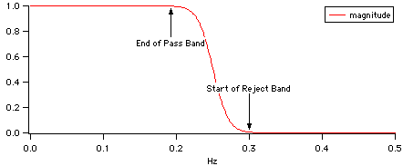
Those frequencies are often expressed as a fraction of the sampling frequency, from 0 to 0.5, the "normalized frequency range" used in classic filter design texts.

It is easier to enter absolute frequencies, though, so you can enter them that way if you set the "Design using this Sampling Frequency (Hz)" value.

You can either directly enter the sampling frequency, or set it by choosing a wave to apply the filter to in the Apply Filter tab:

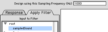
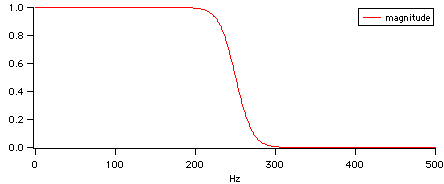
In any event, the design frequencies must be no more than half the sampling frequency . For example, filtering a wave sampled at 1000Hz limits the maximum filter design frequency to 500 Hz.

Design FIR Filter

Design a Finite Impulse Response digital filter by choosing from a combination of low pass, high pass, and notch filtering. The result is a wave containing the combined filter coefficients that can be convolved with waveform data to alter the data's frequency response.

The choice of Window affects mainly the response of the filter in the reject band.

Choose more coefficients to achieve less ripple in the frequency response and better rejection of unwanted frequencies. Odd numbers prevent shifting the filtered result with respect to the input waveform data.

The Notch filter is a maximally-flat high-rejection notch filter centered at approximately the given Notch Frequency. The notch is made very sharp and very rejecting by moving the notch frequency slightly to an advantageous location based on Zahradník and Vlcek's paper as referenced in the FilterFIR command. Click the Response Tab to see the effects of different Notch Width and Improve Notch Accuracy settings.

Design IIR Filter

Design an Infinite Impulse Response digital filter by choosing from a combination of low pass, high pass, and notch filtering. The automatically-designed filter coefficients are bilinear transforms of the Butterworth analog prototype with an optional variable-width notch filter.

More advanced IIR filters (Bessel, Chebyshev) can be designed using the Igor Filter Design Laboratory (IFDL) package. The IIR design software creates IIR coefficients based on bilinear transforms of analog prototype filters such as Bessel, Butterworth, and Chebyshev.

IIR filters can be implemented in 3 different forms: Direct Form 1, Cascade (aka Direct Form II), or Zeros and Poles form. See the FilterIIR command for more details on these implementations.

The cascade implementation is more stable and numerically accurate for high-order IIR filtering than Direct Form I filtering. Cascade IIR filtering is recommended when the filter order exceeds 16 (a 16th-order Direct Form I filter has 17 numerator coefficients and 17 denominator coefficients).

When using the Zeros and Poles implementation, the filter coefficients are complex numbers which define zeros and poles in the (also complex) Z transform domain:

\displaystyle H(z)=\frac{Y(z)}{X(z)}=\frac{\left(z-z_{0}\right) \cdot\left(z-z_{1}\right) \cdot\left(z-z_{2}\right) \cdot \ldots}{\left(z-p_{0}\right) \cdot\left(z-p_{1}\right) \cdot\left(z-p_{2}\right) \cdot \ldots}

The IIR Notch implementation is a simple pole-zero pair placed at the requested notch frequency. The notch depth is controlled by the distance between the pole and zero in the complex plane. Typically the pole p₀ is positioned along the line from the zero z₀ to the origin.

Create Filter using Poles and Zeros Editor

You can create custom IIR filters by manually placing poles and zeros in the Z plane using the Pole and Zero Filter Design procedures, and you can examine the basic IIR filter designs in the Poles and Zeros Editor.

The best way to start designing a filter this way is to modify an automatically-created IIR design. For example, design an IIR notch-only filter with a Notch Frequency of 400 Hz at 50 Hz.

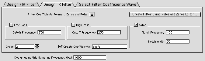
and click the Create Filter using Poles and Zeros Editor... button to display the Poles and Zeros editor:

Here's a pole-zero plot of the 400 Hz / 50 Hz notch implementation:

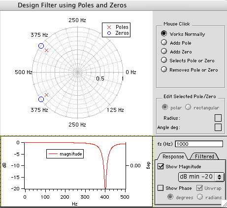
You can manually adjust the pole (X) by clicking it to select it and then adjusting its Radius:

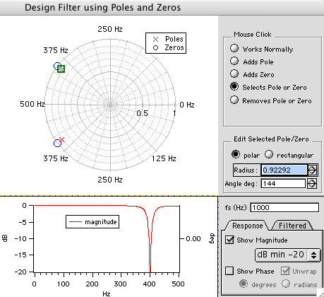
The increased radius brought the pole (and its complex conjugate pole) closer to the zero, which decreased the notch width.

Use the other controls to add, delete, or change poles and zeros. To do this successfully, you should know quite a bit about this kind of filter design.

Select Filter Coefficients Wave

Click the Select Filter Coefficients Wave to select an already-designed filter coefficents wave to apply to data. If the wave is in Zeros and Poles format, it can be edited using the Poles and Zeros editor.

Select the wave to filter in the Apply Filter tab, or view the filter's response in the Resonse Tab.

Response

This tab shows the frequency response of the designed or selected filter in an embedded graph window.

note

"dB" is an engineering abbreviation for "decibels", a unitless ratio. In this filtering context, magnitude in dB is related to gain by: dB= 20*log₁₀(gain). Wikipedia has a nice description here: http://en.wikipedia.org/wiki/Decibel

Apply Filter

Click on the Apply Filter tab select a wave to be filtered (which also sets the filter's sampling frequency). The result of filtering the selected wave is displayed in the graph. Just like a normal graph, you can drag out a marquee in the Response graph, click inside the marquee and choose "Expand" to see more detailed response:

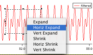
This filtered signal is updated whenever any filter parameter changes. If the filtered wave is large, the time to update the graph will become burdensome; in that case uncheck the Auto-update Filtered Output checkbox and click Update Output Now only when you're ready to wait for the filtering to be done.

Compose Expression Dialog

The Compose Expression dialog provides assistance in generating a command to set the value of a wave, numeric variable or string. This may be helpful while you are "coming up to speed" with Igor. Once you have become familiar with Igor you will probably prefer to enter such commands directly into the command line without the help of this dialog.

The command that you generate with the Compose Expression dialog consists of three parts: the destination, the assignment operator and the expression. The command resembles an assignment and is of the form:

<destination> <assignment operator> <expression>

For example:

wave1 = K0 + wave2         // Wave assignment
K0 += 1.5 * K1             // Variable assignment command
str1 = "Today is" + date() // String assignment command

When the command is composed and you click the Do It button then the expression is evaluated and combined with the destination according to the specified operation.

Select the destination for the command. This is the wave, variable or string which is to be set equal to the expression that you are about to compose.

Select the assignment operator. This determines the way in which the expression is combined with the destination. The simplest assignment operator is "Assign to" in which case the destination's contents are set equal to the expression. For the other assignment operators, the destination's contents are set to the sum, difference, product or quotient of the destination and the expression.

If you click the Create Formula checkbox, Igor uses := as the assignment operator, instead of =. This creates an assignment, called a dependency formula, in which the destination depends on the expression. If any object in the expression changes, Igor will automatically reevaluate the formula and store new values in the destination. See Dependencies for further information. Dependencies create tangled webs that can be confusing and difficult to debug. Consequently, they should be rarely used.

Finally compose the expression by selecting waves, variables, strings, operators and functions from the Insert pop-up menus. You must enter numbers and parentheses from the keyboard.

If you click the Test button, Igor tests the validity of the command that you have generated. If the command is not valid Igor displays an appropriate error message.

Open or Load File Dialog

You can interpret the contents of a file in many ways. Generally, Igor can determine how to open or load a file from the file name extension, and it will simply do that without asking you user about it. Sometimes Igor recognizes that a file (such as a plain text file or a formatted Igor notebook) can be appropriately opened several ways, and will ask you how you want to open it by displaying the Open or Load File Dialog.

note

You can force this dialog to appear by pressing Shift while opening a file through the Recent Files or Recent Experiments menus, or when dropping a file onto the Igor icon.

This is useful for opening an Igor help file as a notebook file for editing.

Select how you want to open the file from the Open As list and then click Open.

When you open a file using the Recent Files or Recent Experiments menus, Igor reopens it as it was previously reopened. Press the Shift key after clicking the File menu but before selecting the file to change how Igor opens the file. For example, if you opened a plain text file as a notebook to examine its contents but you now want to load it as delimited text, click the File menu, then press the Shift key, and then select the file name from the Recent Files menu.

To display the Open or Load File dialog through the Recent Files or Recent Experiments menus, you must click the File menu, then press the Shift key, and then select the file. If you press the Shift key before clicking the File menu, Igor interprets this as an indication that you want to remove the file from the menu.

Load Waves Dialog

The Load Waves dialog generates LoadWave commands that load data from:

Delimited text files
General text files
Fixed field text files
Igor text files
Igor binary wave files

You choose which type of tile to load using the File Type popup menu.

Delimited Text Files

The delimited text file is the most common form of exchange of data from one program to another. In its usual form it consists of rows of numbers separated by tabs or commas with carriage return (CR), linefeed (LF), or carriage return/linefeed combination (CRLF) characters at the end of the row. Often the first row consists of names for each column. Igor attempts to load each column in the file into an Igor wave. There is no limit to the number of rows or columns except that all of the data must fit in available memory.

The delimited text loader can load numeric data, text data, and date/time data. Also, it can handle missing values. If your file contains numeric data only with no missing values, you may find it easier to use the General Text loader, described next.

By default Igor automatically generates wave names of the form wave0, wave1, and so on.

If the Read Wave Names checkbox is checked, Igor looks for column names in the first row. If it finds names it uses them to name the output waves and starts loading data from the next row. If it finds no names, it starts loading data from the first row.

If your file starts with something other than column names or data, for example if it starts with header text, you need to tell Igor where to look for names and data using the Tweaks subdialog, accessed by clicking the Tweaks button.

If the Use File Name in Wave Names checkbox is checked, it overrides the Read Wave Names checkbox. Igor uses the file name minus the extension in the names of the loaded waves. The format of the wave names will be something like <filename><normal name><suffix number>. <normal name> is the name that would be used if Use File Name in Wave Names were unchecked; it is included only if Include Normal Name is checked. <suffix number> is a number appended to make names unique. Depending on the state of the Include Normal Name and Overwrite Existing Waves checkboxes and on whether one or multiple waves are being loaded, <suffix number> may be omitted.

See LoadWave Generation of Wave Names for further discussion of how LoadWave chooses wave names.

Igor cleans up column names, if necessary, so that they are legal standard wave names. The cleanup consists of converting illegal characters into underscores and truncating long names to the maximum of 255 bytes.

By default, Igor attempts to figure out if a column is numeric or text data and creates waves of the appropriate type. You can force interpretation as numeric or text in the Tweaks subdialog.

If Igor encounters a delimiter with no characters preceding it (i.e., two tabs in a row) it takes this as a missing value and stores NaN in a numeric wave or a zero-length string in a text wave.

General Text Files

The general text file format is an Igor invention. It is unique in that it can load multiple "blocks" of data from a file and automatically skips over nonnumeric header text.

The general text loader can load numeric data only. It cannot load text data or date/time data. Also, it cannot handle missing values. If your file contains text data, date/time data, or missing values, load it with the delimited text loader.

A block of data consists of rows of numbers separated by tabs, commas or spaces with carriage return (CR), linefeed (LF), or carriage return/linefeed combination (CRLF) characters at the end of the row. Two or more consecutive rows with the same number of numbers constitute a block. For each block that it finds, Igor attempts to load each column into an Igor wave. There is no limit to the number of blocks, rows or columns except that all of the data must fit in available memory.

The rules for choosing wave names are the same for general text as for delimited text as described above.

Fixed Field Files

The Fixed Field file format is intended to accommodate files written by FORTRAN programs that commonly use columns that have a fixed number of characters in each field. The fields typically use space characters to fill out short fields.

You must specify the number of columns to load, using the Number of Columns control, and the width of each column in bytes, using the Field Widths control. If there are more columns in the file than numbers entered in Field Widths, Igor uses the last number in Field Widths for all remaining columns. Thus, if all columns consist of the same number of bytes, you can enter just one number in the Field Width control.

The fixed field loader, like the delimited text loader, can load numeric data, text data, and date/time data. It can handle missing values. It chooses wave names and identifies the first row containing column names and the first row containing data as described above for the delimited text loader.

Igor Text Files

The Igor text file is a format by which you can transfer not only numeric data but also other information such as wave scaling and units from your custom program into Igor. In addition to data, the Igor text file can contain Igor commands. Thus it is possible for your custom program to generate a file which, when loaded into Igor, will not only create waves but process and display them as well.

By convention the name of an Igor text file has an extension of ".itx".

An Igor text file can contain any number of blocks of waves, each preceded by a WAVES declaration.

If you declare the waves to be complex, Igor uses a pair of numbers in a row for the real and imaginary parts of a each point in the resulting wave.

Igor Binary Wave Files

The Igor binary wave file stores one wave per file. This is the format that Igor uses to save waves that are part of an unpacked Igor experiment. By convention the name of an Igor binary wave file has an extension of ".ibw".

If you want to use a wave in two Igor experiments you will need to load it into the second experiment using Load Igor Binary.

Load Data Tweaks Dialog

The Load Data Tweaks dialog, which you invoke by clicking the Tweaks button in the Load Waves dialog, provides additional options for loading data into Igor.

Delimited Text File Tweaks

If you select "Auto-identify column types" from the Column Types pop-up menu, Igor will attempt to figure out if a column contains numeric data, text data, or date/time data, and will load each column into the appropriate type of wave. You can force interpretation as numeric by selecting "Treat all columns as numeric". Nonnumeric data will be loaded as NaN (Not a Number). If you select "Treat all columns as text", Igor will load even numeric data into text waves as character strings. Such data is not suitable for graphing or analysis.

By default, LoadWave accepts tabs and commas as delimiter characters. You can instruct LoadWave to accept other characters as delimiters. The Tweaks dialog can specify space as a delimiter. The LoadWave command line operation can specify other delimiters as well.

If your file uses spaces to create columns of fixed width (i.e., FORTRAN files), you should use the fixed field loader rather than the delimited text loader.

If space is allowed as a delimiter then Igor treats any number of consecutive spaces as a single delimiter. This means that two consecutive spaces do not indicate a missing value as two consecutive tabs would.

The line numbers that you enter in the various controls are zero-based. The first line in the file is line 0.

General Text File Tweaks

Igor interprets the "Line containing column names" and "First line containing data" tweaks differently for general text files than it does for delimited text files. For delimited text, zero means "first line in the file". For general text, zero for these parameters means auto.

Here is what auto means for general text. If "First line containing data" is auto, Igor starts the search for data from the beginning of the file without skipping any lines. If it is not auto, then Igor skips to the specified line and start its search for data there. Use this to skip a block of data at the beginning of the file. If "Line containing column names" is auto then Igor looks for column names in the line immediately preceding the line found by the search for data. If it is not auto then Igor looks for column names in the specified line.

If the "Number of lines containing data" data tweak is not auto then Igor will stop loading after the first block. This behavior is necessary so that it is possible to pick out a single block or subset of a block from a file containing more than one block.

If a general text file contains more than one block of data and if "Number of lines containing data" is auto then, for blocks after the first one, Igor maintains the relationship between the line containing column names and first line containing data. Thus, if the column names in the first block were one line before the first line containing data then Igor will expect the same to be true of subsequent blocks.

Fixed Field File Tweaks

Fixed field file tweaks are very similar to delimited text file tweaks, but the settings for delimiter characters are missing because fixed field files do not use delimiter characters.

There are two reasons for loading an Igor binary wave file that was created as part of another Igor experiment: You may want your current experiment to share data with the other experiment or you may want to copy data to the current experiment from the other experiment.

In the case of sharing data, you want two experiments to access the same file. If you change the data in the file from one experiment you want it affect the other experiment. In the case of copying data, you want the wave that you load into the second experiment to be independent of wave in the first.

When you load an Igor binary wave file Igor will do one of three things: copy the file into the current experiment, share the file between experiments or ask you which it should do. This is controlled by a setting in the Miscellaneous Settings dialog. Initially it is set to ask you which it should do.

There is a potential problem in sharing a file between two experiments. To see this, imagine that you copy the second experiment to another computer. It is likely that you will forget to copy the .ibw file that the second experiment will need to recreate the wave. When you load the second experiment, you will be irritated when Igor can't fully recreate it. For this reason, it is best to avoid sharing files. You should share files only if you understand this problem and are willing to cope with it. For further discussion, see References to Files and Folders.

Load Image Dialog

The Load Image dialog supports the following image file types:

TIFF
Sun Raster File
Raw PNG
PNG
JPEG
BMP

When you choose a particular type of image file in from the File Type pop-up menu, you are setting a file filter that is used when displaying the image file selection dialog. If you are not sure that your image file has the correct file type or suffix, choose Any from the File pop-up menu so that the filter does not restrict your selection.

There are two ways to load PNG. When Raw PNG is selected, the data is read directly from the file into the wave. When PNG is selected, the file is loaded into memory, and offscreen image is created, and the wave data is set by reading the offscreen image. In nearly all cases, you should choose Raw PNG.

Except for TIFF and SUN Raster images, all images are loaded onto a 3D IGOR wave (unsigned byte with plane 0 containing the red channel, plane 1 the green and plane 2 the blue channel). You can convert the 3D wave into other forms using the ImageTransform operation.

Load General Binary Dialog

The Load General Binary File dialog generates a GBLoadWave command that loads data from a binary file into Igor waves.

Load Excel File Dialog

The Load Excel File dialog generates an XLLoadWave command that loads data from an Excel file into Igor waves.

When you choose the Load Excel File menu item, XLLoadWave displays a dialog that presents a number of options. You should start by clicking the File button. This displays an Open File dialog from which you can select an Excel .xls or .xlsx file. If your Excel file does not appear, choose All Files from the File Types popup menu.

Some programs unfortunately save tab-delimited or other non-Excel type files using the ".xls" extension. If you try to load one of these files, XLLoadWave will tell you that it is not an Excel binary file.

Once you have chosen an Excel file, the main dialog displays the Worksheet popup menu. Choose which worksheet you want to load.

At this point, the From Cell and To Cell edit boxes will display the first and last defined cells in the worksheet. If you want to load just a subset of the entire worksheet, enter the names of the cells in these boxes. The cell names are the same as in Excel: A1 is the top/left cell.

The Columns Types popup menu presents the methods that XLLoadWave can use to decide whether to create a numeric wave or a text wave for a given column in the worksheet. If you are trying to load just numeric data, choose "Treat all columns as numeric". See Column and Wave Types for a discussion of the other methods.

The three radio buttons at the top of the Output Waves section of the dialog determine how XLLoadWave generates names for the new waves. This is discussed above under XLLoadWave and Wave Names.

The Truncate Blanks at End of Columns checkbox matters if your columns have different lengths. This may be because the columns are disparate types of data and there is no reason for them to be the same length. In this case, turn the checkbox on. However, if your columns consist of data sets of the same kind, you should leave this checkbox off. Then XLLoadWave interprets differences in the length of the columns as due to blank cells at the end of some of them. All of the loaded waves will contain the same number of points but with different numbers of blanks at the end.

The Discard Waves with Fewer Than item controls how XLLoadWave decides whether to keep a wave or not. This item allows you to set the minimum number of points. XLLoadWave will skip creating waves that have fewer than the number of points that you enter.

Load Matlab MAT File Dialog

The Load Matlab MAT File dialog generates an MLLoadWave command that loads data from a Matlab MAT file into Igor waves.

Find 64-bit Matlab

To read Matlab .mat data files Igor needs to link to dynamic libraries that come with Matlab.

See Loading Matlab MAT Files for further information.

Load JCAMP-DX File Dialog

The Load JAMP-DX File dialog generates a JCAMPLoadWave command that loads data from a JCAMP-DX file into Igor waves.

Save Waves Dialog

You can save waves to a file in delimited text, general text, Igor text or in Igor binary format.

Since waves are automatically saved when you save the Igor experiment that they are part of, you may never need these operations. They are useful if you want to create an additional file for export to another program or to a different Igor experiment.

When exporting to another program, delimited text is usually the best choice.

For making a copy of one or a few Igor waves that you want to open in a different Igor experiment, use Igor binary format. In most cases you will want to select Save a Copy. If you select Relocate to File then the new file, where ever it is, will become part of the experiment and when you save the experiment then this wave will be saved in this new file. Sometimes that is what you want, sometimes not. See References to Files and Folders for details.

Igor text format is convenient for saving a number of Igor waves in one file to be opened from a different Igor experiment.

Only one wave can be saved in a single Igor binary wave file.

Select the name of a symbolic path from the Path list if there is a symbolic path that identifies the folder in which you want to save the file. If you select no symbolic path or you enable the Interactive checkbox Igor will present you with a standard save dialog to allow you to specify the folder and name of the file to save.

When Igor saves waves of different lengths as general text it writes all waves of the same length in a block of data. All waves in a given block will have the same number of points. When Igor writes a delimited text file it writes a single block only. If the waves have different lengths then some columns will have missing values at the end.

The exact action taken upon a binary save depends both on the settings in this dialog and on the history of the wave:

If the wave was loaded from (and is still connected to) a binary file,

and if you do not specify a path,
and you do not enable the Interactive checkbox,
and you do not select Save a Copy,

then the wave will be written back to the file from which it came.

Otherwise a Save File dialog will be displayed in which you can choose the new file location.

For greater control of the formatting of delimited text and general text files you can use the Use Table Formatting option. This takes the formatting for each wave from the top table, if any. Start by creating a table containing the waves you want to save. Be sure to display enough digits in the table because the data will be written to the file as it appears in the table. When saving a multi-column wave (1D complex wave or multi-dimensional wave), all columns of the wave are saved using the table format for the first table column from the wave.

New Symbolic Path Dialog

Enter the name of the new symbolic path in the Name entry. Then click the Path button. Igor presents a Choose Folder dialog in which you can choose the folder to which the symbolic path is to refer.

A list of all symbolic paths show up in the various Load and Save dialogs.

Igor automatically creates symbolic paths when you do something that makes the current experiment depend on a file stored outside of the experiment, for example, when you load an Igor binary data file. These automatically-created symbolic paths help Igor find the file when you next open the experiment.

Symbolic Path Status Dialog

When you select a symbolic path from the Symbolic Path list, any Igor objects that were loaded from the selected path are displayed in the Objects from Path list.

If you select the _none_ item in the path list then the Objects from Path list shows the objects that were not loaded from any folder. This includes the built-in procedure window, any waves that have not yet been saved to disk and any waves, notebooks or procedure files that are stored in packed experiment files.

Kill Symbolic Paths Dialog

The Kill Symbolic Paths dialog lists all symbolic paths that are not in use. A path is "in use" if the folder that it refers to contains a file that would be needed to recreate the current experiment.

Igor automatically creates a symbolic path when you load a file from a folder that is not part of the current experiment - for example, if you open a procedure file from another experiment. If you kill that procedure file, then the path will not longer be in use. However, Igor will not automatically kill the path since you may want to use it again. If you do this a number of times, you may wind up with a number of paths that are not really needed. You can use this dialog to get rid of them.

Overwrite or Delete Folder

This dialog is presented when a MoveFolder or CopyFolder operation is about to overwrite an existing folder on disk or when a DeleteFolder operation is about to delete a folder on disk. This is intended to prevent accidental or malicious deletion of data.

You can give or deny permission to overwrite or delete the folder by clicking the appropriate dialog button. If you deny permission, the operation returns an error to the calling user-defined function.

If you want to grant blanket permission to overwrite or delete folders, use the Miscellaneous section of the Miscellaneous Settings dialog, accessible via the Misc menu. Doing so increases the risk of accidental or malicious deletion of files so you should exercise caution.

Simple Input Dialog

Missing Parameter Dialog

If a macro is invoked with missing parameters or if a DoPrompt command is executed in a user-defined function, Igor displays this dialog to ask you to enter parameter values.

If the you enter the parameters and click the Continue button then execution continues. If you click Cancel or Quit Macro, executions stops.

New Page Layout Dialog

The New Page Layout dialog creates a new page layout window consisting of one page. You can add other pages using Layout→Page→Add Page after creating the layout window.

You can create a layout with no objects in it by clicking Do It without selecting any objects. You can append objects to the layout later.

Style macros provide a way to apply predefined styles to new layouts. You must first define your style macro. You can then apply it by choosing its name from the Style popup menu. See Page Layout Style Macros for details.

Append Objects Dialog

There is no difference between appending a graph or table using this dialog and appending it using the Graph pop-up menu or Table pop-up menu in the layout's control panel.

Use the Layout→Add Annotation to add a textbox to the layout.

To place a picture in the layout, paste it from the Clipboard or use Misc→Pictures.

Remove Objects Dialog

Although you can append only graph or table type objects using the Append to Layout dialog, you can remove any type object using the Remove from Layout dialog.

You can also remove an object by selecting it and pressing Delete or selecting the Clear or Cut items from the Edit menu. You can clear or cut multiple objects by using the marquee tool in the layout's control panel. First, click on the marquee tool. Next, marquee the objects to be cleared or cut. Finally, click inside the marquee and select Clear or Cut from the pop-up menu.

Modify Objects Dialog

Normally you reach this dialog by choosing Layout→Modify Objects or by double-clicking layout object. Double-clicking in Left, Top, Width, or Height areas in the info panel also summons this dialog.

An object's left and top coordinates are relative to the top left corner of the entire page, including margins.

To modify an annotation's content, click the annotation with the text tool.

Arrange Objects Dialog

If you want to arrange objects in a certain area of the layout, select the marquee tool and marquee the area where you want the objects to go before choosing Layout→Arrange Objects dialog. Then make sure the "Use marquee" checkbox is selected. If there is no marquee when you select Arrange Objects or if the "Use marquee" checkbox is unchecked, then the objects will be arranged in the entire page.

If you select no objects in the list and all of the checkboxes are unchecked, then all of the objects in the layout are arranged.

The order in which objects are tiled is determined by the order in which they appear in the command generated by the Arrange Objects dialog. This in turn depends on the front-to-back ordering of the objects in the layout. Objects are tiled from left to right, top to bottom. Therefore, you can control exactly where each object winds up by controlling the front to back ordering. Another approach is to use the Arrange Objects dialog to compose the Tile command. Then, instead of clicking Do It, click To Cmd Line, putting the Tile command in the command line. Now, arrange the objects in the command line in the order in which you want them tiled. Then press Return to execute the Tile command.

Layout Page Size Dialog

In Igor Pro 6 and earlier versions, the layout page size was controlled using the system Page Setup dialog. Now each layout has its own size setting that is independent of the page setup. We made this change because printing is much less common now than when page layouts were originally designed, decades ago. It is more common now for people to create graphics for display in a web page or for embedding in a journal paper. For these purposes, you usually need to control the size of the graphics independent of any paper size.

Settings for All Slide Shows Dialog

A layout slide show is a full-screen display of the pages in a layout, suitable for a presentation to a group. You start a slide shows by clicking the button at the bottom/right corner of the layout page sorter, or using the LayoutSlideShow operation.

Using the Slide Show Settings dialog, you can control various aspects of the slide show, including:

How pages are scaled to fit the screen

How multiple monitors are used

The time to wait before showing the next slide

Make Plot Areas Uniform Dialog

The Make Plot Areas Uniform dialog sets the margins and plot areas of the selected graphs to uniform values so that the axes in the graphs can be aligned. For a detailed example, see Aligning Layout Objects.

Select the graphs that you want to make uniform in the list.

If you are stacking graphs vertically, you need to make the horizontal plot areas uniform, so choose Horizontally from the Make Plot Areas Uniform pop-up menu. If you are stacking horizontally, choose Vertically from the pop-up menu. In this discussion, we will assume that you are making the plot areas uniform horizontally.

Normally you will want to set all three of the values: left margins, right margins, and plot area widths, so make sure all three checkboxes are checked. Then click each of the Estimate buttons to find the approximately correct values.

The estimated values are determined from the graph windows associated with the selected graph objects in the list. The estimated left margin is the largest left margin of the graph windows, the estimated right margin is the largest right margin of the graph windows, and the estimated width is the largest width of the graph windows.

Now click Do It. After examining the layout, you may need to revisit this dialog to tweak the values.

Make the horizontal plot ares uniform does not guarantee that the vertical axes will line up. This is because of the axis standoff setting. You may want to turn axis standoff off for each graph, using Graph→Modify Axis dialog.

This dialog generates ModifyGraph commands that affect the margins and width or height of the graph windows associated with the selected graph objects. If you want to restore a graph window to its original state, you need to activate the windows and use Graph→Modify Graph to reset the appropriate settings.

Draw Environment Dialog

The Modify Draw Environment dialog appears when you choose All from the Draw Environment pop-up menu icon (tree and grass). It also appears when you select an object with the arrow tool, right-click, and choose All.

If you invoke the dialog with one or more drawing objects selected, it changes the properties of the selected objects.

If you invoke the dialog with no drawing objects selected, it affects objects that you subsequently create.

See also: Drawing for a complete discussion

Create Draw Object Dialog

The Create Draw Object dialog appears when you click and hold on an object icon (e.g., rectangle) in the drawing tool palette and choose the Create item (e.g., Create Rectangle) from the resulting pop-up menu.

Use this dialog to create a drawing object by entering numerical coordinates and setting the other properties.

Modify Draw Object Dialog

The Modify Draw Object dialog appears when you double-click a drawing object with the arrow tool selected in the drawing tool palette.

Use this dialog to change the properties of an object including the defining coordinates. You will get a similar dialog but without the coordinate values if you double-click a group of objects.

You can also change the properties of a selected object by choosing items from the Draw Environment pop-up menu icon (tree and grass) or right-clicking and using the resulting contextual pop-up menu.

Notebook Action Dialog

A notebook action is a special character which, when clicked, executes Igor commands. The action can display a title, a picture, or both.

The procedure picture feature is for advanced Igor users. It allows the picture for an action to come from an Igor procedure file.

If you use a picture, you should convert it to PNG which is a cross-platform bitmap format. Procedure picture are always PNG.

Notebook Action Helper File Dialog

This feature is for advanced Igor users. It designates a procedure file associated with a notebook. The procedure file is automatically opened. It may contain functions and/or procedure picture used by actions in the notebook.

Convert to UTF-8 Text Encoding Dialog

You may want to convert old files that use non-UTF-8 text encodings to UTF-8. For example, if you are exporting data to another program, you may want to convert to UTF-8 for compatibility. The Convert to UTF-8 Text Encoding dialog facilitates such conversions. See Converting to UTF-8 for details.

Text Magnification Dialog

You can enter a text magnification between 25 and 500 percent.

Normally it will be sufficient to choose a predefined text magnification from the magnification icon in the bottom/left corner of the window or using the Magnification submenu in the contextual menu for the window. To display the contextual menu, right-click in the body of the window.

Gizmo Movie Dialog

The Gizmo Movie Panel helps you to create a basic movie from a Gizmo display.

A movie is composed of any sequence of frames captured from a Gizmo window. You can add the frames manually or have them added sequentially for a selected type of rotation. All frames must be of the same size so don't change the size of the Gizmo window while your movie file is open.

Before you open a new movie file you need to specify the desired frame rate. The frame rate can't be changed after you open the movie file for writing.

Click the New Movie button to specify the movie file location on disk. When the file is opened the button changes to Finish Movie. Click Finish Movie to close the movie file and save all the frames that you added.

After you opened the movie file you can modify the display in Gizmo, keeping the window size fixed, and click the Append Single Frame button to add one frame at a time.

If you want to add a range of frames, start by specifying the number of frames that you want to add and then choose the type of rotation. Uniform rotation about an axis adds the specified number of frames from the current orientation to span the specified number of degrees. You can drag the slider between the start and end markers to see the range of rotation that will be added.

When you choose Spherical Linear Interpolation (SLERP), you need to specify both the start and the end orientations. To do so, first rotate the Gizmo plot to the desired starting orientation and click the left From Gizmo button. Then rotate Gizmo plot to the desired ending position orientation and click the right From Gizmo button. Use the slider to make sure that the rotation covers the desired range of rotation.

Click Append Rotation Frames to add the specified number of frames to the movie. You can add frames to the movie from multiple rotations.

When you have finished adding all the frames that you want in your movie, click Finish Movie. Nothing is saved until you click this button.

License Installation Dialog

The License Installation dialog appears only after clicking "Activate Entered License" when the "Install License for All Users" checkbox is checked:

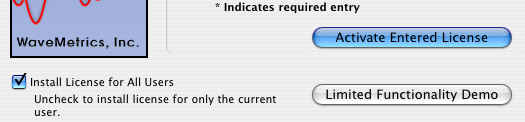
There are two ways to install a license for use by multiple users:

For all local users of this computer
For all local and remote users of this server (server installation)

The first choice is appropriate if you are installing Igor on a single-user computer (with possibly multiple login accounts), or you are sharing Igor with other users so that only one copy of Igor is in use at any time.

The second is appropriate if you are installing a multi-user license (in which case the dialog's wording changes a little to indicate it is the preferred choice):

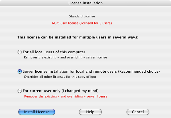
A server license installation allows a user on another computer using network access to use the Igor installed on the current computer without needing to re-enter the license serial number and activation key.

A third choice is presented:

For current user only

This last option is recommended for owners of a single-user Igor license with only one login account.

For all choices, it is the responsibility of those using Igor to limit the concurrent users of Igor to the number specified by the Igor license.

The comments below each radio button about removing existing licenses refers to the consequences of clicking "Install License".

There is a hierarchy of licensing: a server license "trumps" (or overrides) a license for the current user only, which in turn overrides a license for all local users.

In order to install a lower priority license, the higher priority licenses must be removed. This dialog does not appear unless Igor thinks it is possible to remove them.

Two Samples Tests

Choose Statistics→Two Sample Tests to display the Two Sample Tests control panel. The panel performs statistics tests on two waves. See Tests For Two Waves for the list of two-wave tests.

The Two Sample Tests control panel is designed to assist you in selecting hypothesis tests for two populations. The results of your selections at each stage are saved in an IGOR notebook. You should examine these results to determine how to proceed after each step. The procedure suggests a conclusion following each test but it is left to you to make the final determination. It is therefore a good idea to inspect the intermediate results printed in the notebook. This is particularly important in cases where the outcome of a test is not conclusive.

Use the Next and Back buttons to navigate between steps of the process. You can back-track at any stage and try a different route to investigate other options.

All the results of the analysis are contained in the notebook but should you want to explore them further you can find the waves created by the various tests in the data folder root:Packages:TSP.

The following sections describe the control panel's tabs.

General

In this tab you specify the type of data that you intend to explore. Choices are Ratio, Ordinal or Nominal data. Both ratio and ordinal expect real numeric input while Nominal works on both numeric and text waves. The two populations may be dependent (in which case you should check the Paired Samples checkbox) or independent. A general alpha (confidence) level is set here for use in all subsequent tests.

Data Selection

In this tab you select the two waves containing the two populations to be tested. The waves should generally be 1D real numeric waves. Text waves are also supported for nominal data input.

Step 1

Ratio Data

You can use this tab to test if the two samples are random and normally distributed.

Ordinal Data

This step is skipped.

Nominal Data

You can use this step to perform a non-parametric Runs test (StatsNPNominalSRTest). Note that this test is designed for data containing two types and so it should be skipped if your samples contain three or more types.

Step 2

Unpaired ratio data

You should test if the variances are equal. If the variances are not equal you should continue with a non-parametric test (Wilcoxon).

Paired ratio data

You should run a t-test at this step.

Unpaired ordinal data

Run the non-parametric Wilcoxon test.

Paired ordinal data

Run the Wilcoxon signed test.

Step 3

This step applies only to unpaired ratio data. It is used to run the t-test.

Dialog Overview​

Operation Dialogs​

Dialog Wave Browser​

Operation Result Chooser​

Operation Result Displayer​

Dialog Help​

Macro Errors During Experiment Load​

Missing Folder Dialog​

Skip All Waves From Missing Folder Dialog​

Missing Wave File Dialog​

Missing File Dialog​

Loading General Text Dialog​

Save Graphics File Dialog​

Choose Text Encoding Dialog​

Resolve Text Encoding Conflict Dialog​

Export Graphics Dialog​

Substitute Font Dialog​

Edit Font Substitution Dialog​

Default Font Dialog​

Pictures Dialog​

Adopt Window Dialog​

Object Status Dialog​

Rename Objects Dialog​

Make Waves Dialog​

Kill Waves Dialog​

Duplicate Waves Dialog​

Change Wave Scaling Dialog​

Redimension Waves Dialog​

Insert Points Dialog​

Delete Points Dialog​

New Graph Dialog​

Remove from Graph Dialog​

Modify Graph Dialog​

New Box Plot Dialog​

Append Box Plot Dialog​

Modify Box Plot Dialog​

New Violin Plot Dialog​

Append Violin Plot Dialog​

Modify Violin Plot Dialog​

New Category Plot Dialog​

Append Category Traces Dialog​

New Contour Plot Dialog​

Append Contour Plot Dialog​

Modify Contour Appearance Dialog​

More Contour Levels Dialog​

Contour Line Colors Dialog​

Contour Labels Dialog​

New Image Plot Dialog​

Append Image Plot Dialog​

Reorder Images Dialog​

Modify Image Appearance Dialog​

Append Traces Dialog​

Reorder Traces Dialog​

Modify Trace Appearance Dialog​

Trace Offset Dialog​

Replace Wave Dialog​

Modify Axis Dialog​

Error Bars Dialog​

Set as f(z) Dialog​

Text Markers Dialog​

Dashed Lines Dialog​

Add Annotation Dialog​

New Table Dialog​

Append Columns to Table Dialog​

Remove Columns from Table Dialog​

Modify Columns Dialog​

Set Overall Dimension Labels Dialog​

Set Dimension Label Dialog​

Tile or Stack Windows Dialog​

Close Window Dialog​

Window Control Dialog​

Control Bar Dialog​

Button Control Dialog​

CheckBox Control Dialog​

ValDisplay Control Dialog​

PopupMenu Control Dialog​

SetVariable Control Dialog​

Slider Control Dialog​

Tab Control Dialog​

TitleBox Control Dialog​

Dialog Overview

Operation Dialogs

Dialog Wave Browser

Operation Result Chooser

Operation Result Displayer

Dialog Help

Macro Errors During Experiment Load

Missing Folder Dialog

Skip All Waves From Missing Folder Dialog

Missing Wave File Dialog

Missing File Dialog

Loading General Text Dialog

Save Graphics File Dialog

Choose Text Encoding Dialog

Resolve Text Encoding Conflict Dialog

Export Graphics Dialog

Substitute Font Dialog

Edit Font Substitution Dialog

Default Font Dialog

Pictures Dialog

Adopt Window Dialog

Object Status Dialog

Rename Objects Dialog

Make Waves Dialog

Kill Waves Dialog

Duplicate Waves Dialog

Change Wave Scaling Dialog

Redimension Waves Dialog

Insert Points Dialog

Delete Points Dialog

New Graph Dialog

Remove from Graph Dialog

Modify Graph Dialog

New Box Plot Dialog

Append Box Plot Dialog

Modify Box Plot Dialog

New Violin Plot Dialog

Append Violin Plot Dialog

Modify Violin Plot Dialog

New Category Plot Dialog

Append Category Traces Dialog

New Contour Plot Dialog

Append Contour Plot Dialog

Modify Contour Appearance Dialog

More Contour Levels Dialog

Contour Line Colors Dialog

Contour Labels Dialog

New Image Plot Dialog

Append Image Plot Dialog

Reorder Images Dialog

Modify Image Appearance Dialog

Append Traces Dialog

Reorder Traces Dialog

Modify Trace Appearance Dialog

Trace Offset Dialog

Replace Wave Dialog

Modify Axis Dialog

Error Bars Dialog

Set as f(z) Dialog

Text Markers Dialog

Dashed Lines Dialog

Add Annotation Dialog

New Table Dialog

Append Columns to Table Dialog

Remove Columns from Table Dialog

Modify Columns Dialog

Set Overall Dimension Labels Dialog

Set Dimension Label Dialog

Tile or Stack Windows Dialog

Close Window Dialog

Window Control Dialog

Control Bar Dialog

Button Control Dialog

CheckBox Control Dialog

ValDisplay Control Dialog

PopupMenu Control Dialog

SetVariable Control Dialog

Slider Control Dialog

Tab Control Dialog

TitleBox Control Dialog