Contour Plots

A contour plot is a two-dimensional XY plot of a three-dimensional XYZ surface showing lines where the surface intersects planes of constant elevation (Z).

One common example is a contour map of geographical terrain showing lines of constant altitude, but contour plots are also used to show lines of constant density or brightness, such as in X-ray or CT images, or to show lines of constant gravity or electric potential.

The contour plot is appropriate for data sets of the form:

z= f(x,y)

meaning there is only one Z value for each XY pair. This rules out 3D shapes such as spheres, for example.

Contour Data

You can create contour plots from two kinds of data:

Gridded data stored in a matrix
XYZ triplets

Gridded Data

Gridded data is stored in a 2D wave, or "matrix wave". By itself, the matrix wave defines a regular XY grid. The X and Y coordinates for the grid lines are set by the matrix wave's row X scaling and column Y scaling.

You can also provide optional 1D waves that specify coordinates for the X or Y grid lines, producing a nonlinear rectangular grid like the one shown here. The dots mark XY coordinates specified by the 1D waves:

Contouring gridded data is computationally much easier than XYZ triplets and consequently much faster.

XYZ Data

XYZ triplets can be stored in a matrix wave of three columns, or in three separate 1D waves each supplying X, Y, or Z values. You must use this format if your Z data does not fall on a rectangular grid. For example, you can use the XYZ format for data on a circular grid or for Z values at random X and Y locations.

XYZ contouring involves the generation of a Delaunay triangulation of your data, which takes more time than is needed for gridded contouring. You can view the triangulation by selecting the Show Triangulation checkbox in the Modify Contour Appearance dialog.

For best results, you should avoid having multiple XYZ triplets with the same X and Y values. If the contour data is stored in separate waves, the waves should be the same length.

If your data is in XYZ form and you want to convert it to gridded data, you can use the ContourZ function on an XYZ contour plot of your data to produce a matrix wave. The AppendImageToContour procedure in the WaveMetrics Procedures folder produces such a matrix wave, and appends it to the top graph as an image. Also see the Voronoi parameter of the ImageInterpolate operation for generating an interpolated matrix.

Creating a Contour Plot

Contour plots are appended to ordinary graph windows. All the features of graphs apply to contour plots: axes, line styles, drawing tools, controls, etc. See Graphs.

You can create a contour plot in a new graph window by choosing Windows→New→Contour Plot. This displays the New Contour Plot dialog. This dialog creates a blank graph to which the plot is appended.

To add a contour plot to an existing graph, choose Graph→Append To Graph→Contour Plot. This displays the Append Contour Plot dialog.

You can also use the AppendMatrixContour or AppendXYZContour operations.

You can add a sense of depth to a gridded contour plot by adding an image plot to the same graph. To do this, choose Graph→Append To Graph→Image Plot. This displays the Append Image Plot dialog. If your data is in XYZ form, use the AppendImageToContour WaveMetrics procedure to create and append an image.

These commands generate a gridded contour plot an image plot:

Make/O/D/N=(50,50) mat2d				// Make some data to plot
SetScale x,-3,3,mat2d
SetScale y,-3,3,mat2d
mat2d =  3*(1-y)*(1-y) * exp(-(x*x) - (y+0.5)*(y+0.5))
mat2d -= 8*(x/5 - x*x*x - y*y*y*y*y) * exp(-x*x-y*y) 
mat2d -= 1/4 * exp(-(x+.5)*(x+.5) - y*y)
Display;AppendMatrixContour mat2d		// Creates the contour plot
AppendImage mat2d

Instead of displaying an image plot with the contour plot, you can instruct Igor to add a color fill between contour levels. You can see this using these commands:

RemoveImage mat2d
ModifyContour mat2d ctabFill={*,*,Grays256,0}

Modifying a Contour Plot

You can change the appearance of the contour plot by choosing Graph→Modify Contour Appearance. This dialog is also available as a subdialog of the New Contour Plot and Append Contour Plot dialogs.

You can open the Modify Contour Appearance dialog by Shift-double-clicking the contour plot or by right-clicking it but not on a contour and choosing Modify Contour Appearance from the contextual menu.

Use preferences to change the default contour appearance, so you won't be making the same changes over and over. See Contour Plot Preferences.

The Modify Contour Appearance Dialog

The following sections describe some of the contour plot parameters you can change with the Modify Contour Appearance dialog.

The Contour Data pop-up menu shows the "contour instance name" of the contour plot being modified. The name of the contour plot is the same as the name of the Z wave containing the contour data.

If the graph contains more than one contour plot, you can use this pop-up menu to change all contour plots in the target graph.

If the graph contains two contour plots using the same Z wave name, an instance number is appended to those Z wave names in this pop-up menu. See Instance Notation and Contour Instance Names.

Contour Levels

Each contour trace draws lines at one constant Z level. The Z levels are assigned automatically or manually as specified in this part of the dialog.

Igor computes automatic levels by subdividing the range of Z values into approximately the number of requested levels. You can instruct Igor to compute the Z range automatically from the minimum and maximum of the Z data, or to use a range that you specify in the dialog. Igor attempts to choose "nice" contour levels that minimize the number of significant digits in the contour labels. To achieve this, Igor may create more or fewer levels than you requested.

You can specify manual levels directly in the dialog in several ways:

Linearly spaced levels (constant increment) starting with a first level and incrementing by a specified amount.
A list of arbitrary levels stored in a wave you choose from a pop-up Wave Browser.
A list of arbitrary levels you enter in the More Contour Levels dialog that appears when you click the More Contour Levels checkbox. These levels are in addition to automatic, manual, or from-wave levels.

The More Contour Levels dialog can be used for different purposes:

To add a contour level to those already defined by the automatic, manual, or from-wave levels. You might do this to indicate a special feature of the data.
As the only source of arbitrary contour levels, for complete control of the levels. You might do this to slightly change a contour level to avoid problems (see Contouring Pitfalls). Disable the auto or manual levels by entering 0 for the number of levels. The only contour levels in effect will be those entered in the More Contour Levels dialog.

WaveMetrics provides some procedures for dealing with contour levels. See WaveMetrics Contour Plot Procedures for details.

Igor normally recalculates and redraws the contour plot whenever any change occurs that might alter its appearance. This includes changes to any data waves and the wave supplying contour levels, if any. Since calculating the contour lines can take a long time, you may want to disable this automatic update with the Update Contours pop-up menu.

"Off" completely disables updating of the contours for any reason. Choose "once, now" to update the contour when you click the Do It button. "Always" selects the default behavior of updating whenever the contour levels change.

Igor normally adds labels to the contour lines, and updates them whenever the contour lines change (see Update Contours Pop-Up Menu). Since updating plots with many labels can take a long time, you may want to disable or modify this automatic update with the Labels pop-up menu.

"None" removes any existing contour labels, and prevents any more from being generated.

"Don't update any more" keeps any existing labels, and prevents any more updates. This is useful if you have moved, removed, or modified some labels and you want to keep them that way.

"Update now, once" will update the labels when you click the Do It button, then prevents any more updates. Use this if updating the labels takes too long for you to put up with automatic updates.

"If contours change", the default, updates the labels whenever Igor recalculates the contour lines.

"Always update" is the most aggressive setting. It updates the labels if the graph is modified in almost any way, such as changing the size of the graph or adjusting an axis. You might use this setting temporarily while making adjustments that might otherwise cause the labels to overlap or be too sparse.

Click Label Tweaks to change the number format and appearance of the contour labels with the Contour Labels dialog. See Modifying Contour Labels.

For more than you ever wanted to know about contour labels, see Contour Labels.

Line Colors Button

Click the Line Colors button to assign colors to the contour lines according to their Z level, or to make them all the same color, using the Contour Line Colors dialog.

Autoscaled color mapping assigns the first color in a color table to the minimum Z value of the contour data (not to the minimum contour level), and the last color to the maximum Z value. To see what the color tables look like, see Color Table Details.

See The Color of Contour Traces for further discussion of contour colors.

Show Boundary Checkbox

Click this to generate a trace along the perimeter of the contour data in the XY plane. For a matrix contour plot, the perimeter is simply a rectangle enclosing the minimum and maximum X and Y. The perimeter of XYZ triplet contours connects the outermost XY points. This trace is updated at the same time as the contour level traces.

Show XY Markers Checkbox

Click this to generate a trace that shows the XY locations of the contour data. For a matrix contour plot, the locations are by default marked with dots. For XYZ triplet contours, they are shown using markers. As with any other contour trace, you can change the mode and marker of this trace with the Modify Trace Appearance dialog. This trace is updated at the same time as the contour level traces.

Fill Contours Checkbox

Click this to fill between contour levels with solid colors. Click the Fill Colors button to adjust the colors in the same manner described under Line Colors Button.

warning

Solid fills can sometimes fail.

You can set the fill and color for individual levels using the Modify Trace Appearance dialog even if the Fill Contours Checkbox is off.

See Contour Fills for more information.

Show Triangulation Checkbox

Click this to generate a trace that shows the Delaunay triangulation of the contour data. This is available only for XYZ triplet contours. This trace is updated at the same time as the contour level traces.

XYZ triplet contours can be interpolated to increase the apparent resolution, resulting in smoother contour lines. The interpolation uses the original Delaunay triangulation. Increasing the resolution requires more time and memory; settings higher than x16 are recommended only to the very patient.

Contour Traces

Igor creates XY pairs of double-precision waves to contain the contour trace data, and displays them as ordinary graph traces. Each trace draws all the curves for one Z level. If a single Z level generates more than one contour line, Igor uses a blank (NaN) at the end of each contour line to create a gap between it and the following line.

The same method is used to display markers at the data's XY coordinates, the XY domain's boundary, and, for XYZ triplet contours only, the Delaunay triangulation.

The names of these traces are fabricated by Igor from the name of the Z data wave or matrix. See Contour Trace Names.

One important special property of these waves is that they are private to the graph. These waves do not appear in the Data Browser or in any other dialog, and are not accessible commands. There is a trick you can use to copy these waves, however. See Extracting Contour Trace Data.

The contour traces, which are the visible manifestation of these private waves, do show up in the Modify Trace Appearance dialog, and can be named in commands just like other traces.

There is often no need to bother with the individual traces of a contour plot because the Modify Contour Appearance dialog provides adequate control over the traces for most purposes. However, if you want to distinguish one or more contour levels, to make them dashed lines, for example, you can do this by modifying the traces using the Modify Trace Appearance dialog. For further discussion, see Overriding the Color of Contour Traces.

Contour Trace Names

The name of a contour trace is usually something like "zwave=2.5", indicating that the trace is the contour of the z data set "zwave" at the z=2.5 level. A name like this must be enclosed in single quotes when used in a command:

ModifyGraph mode('zwave=2.5')=2

This trace naming convention is the default, but you can create a different naming convention when you first append a contour to a graph using the /F flag with AppendMatrixContour or AppendXYZContour. The contour dialogs do not generate /F flags and therefore create contours with default trace names. See the AppendMatrixContour operation and the AppendXYZContour operation for a more thorough discussion of /F.

Example: Contour Legend with Numeric Trace Names

To make a legend contain slightly nicer wording you can omit the "zwave=" portion from trace names with /F="%g":

AppendMatrixContour/F="%g" zw	// trace names become just numbers

/F="%s=%g" (default) /F="%g"

You can manually edit the legend text to remove the single quotes around the trace names. Double-click the legend to bring up the Modify Annotation dialog.

For details on creating contour plot legends, see Contour Legends.

Contour Trace Programming Notes

The TraceNameList function returns a string which contains a list of the names of contour traces in a graph. You can use the name of the trace to retrieve a wave reference for the private contour wave using TraceNameToWaveRef. See also Extracting Contour Trace Data.

If a graph happens to contain two traces with the same name, Igor uses "instance notation" to tell them apart. For example, two traces named "2.5" would show up in the Modify Trace Appearance dialog as "2.5" and "2.5#1". On the command line, you would use something like:

ModifyGraph mode('2.5'#1)=2

Notice how the instance notation (the "#1" part) is outside the single quotes. This instance notation is needed when the graph contains two contour plots that generate identically named traces, usually when they use the same /F parameters and draw a contour line at the same level (z=2.5).

See Instance Notation. Also see Contour Instance Names.

The Color of Contour Traces

By default, contour traces are assigned a color from the Rainbow color table based on the contour trace's Z level. You can choose different colors in the Contour Line Colors subdialog of the Modify Contour Appearance dialog.

The Contour Line Colors dialog provides three choices for setting the contour trace colors:

All contour traces can be set to the same color.
The color for a trace can be selected from a "color index wave" that you created, by matching the trace's Z level with the color index wave X index.
The color for a trace can be computed from a chosen built-in color table or from a color table wave that you created, by matching the trace's Z level with the range of available colors.

Color Tables

When you use a color table to supply colors, Igor maps the Z level to an entry in the color table. By default, Igor linearly maps the entire range of Z levels to the range of colors in the table by assigning the minimum Z value of the contour data to the first color in the table, and the maximum Z value to the last color:

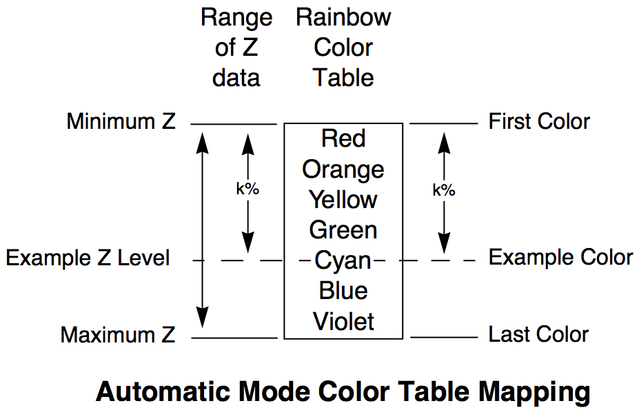
With the Modify Contour Appearance dialog, you can assign a specific Z value to the color table's first and last colors. For example, you can use the first half of the color table by leaving First Color on Auto, and typing a larger number (2*(ZMax-ZMin), to be precise) for the Last Color.

To see what the built-in color tables look like, see Color Table Details.

You can create your own color table waves that act like custom color tables. See Color Table Waves for details.

Color Index Wave

You can create your own range of colors by creating a color index wave. The wave must be a 2D wave with three columns containing red, green, and blue values that range from 0 (zero intensity) to 65535 (full intensity), and a row for each color. Igor finds the color for a particular Z level by choosing the row in the color index wave whose X index most closely matches the Z level.

To choose the row, Igor converts the Z level into a row number as if executing:

colorIndexWaveRow= x2pnt(colorIndexWave,Z)

which rounds to the nearest row and limits the result to the rows in the color index wave.

When the color index wave has default X scaling (the X index is equal to row number), then row 0 contains the color for z=0, row 1 contains the color for z=1, etc. By setting the X scaling of the wave (Change Wave Scaling dialog), you can control how Igor maps Z level to color. This is similar to setting the First Color and Last Color values for a color table.

Color Index Wave Programming Notes

Looking up a color in a color index wave can be expressed programmatically as:

red=   colorIndexWave (Z level)[0]
green= colorIndexWave (Z level)[1]
blue=  colorIndexWave (Z level)[2]

where ( ) is used to index into rows using X scaling, and [ ] selects a column using Y point number (column number).

Here is a code fragment that creates a color index wave that varies from blue to red:

Function CreateBlueRedColorIndexWave(numberOfColors,zMin,zMax)
	Variable numberOfColors
	Variable zMin,zMax		// From min, max of contour or image data
	
	Make/O/N=(numberOfColors,3) colorIndexWave
	Variable white = 65535						// black is zero
	Variable colorStep = white / (numberOfColors-1)
	
	colorIndexWave[][0]= colorStep*p					// red increases with row number,
	colorIndexWave[][1]= 0			// no green
	colorIndexWave[][2]= colorStep*(numberOfColors-1-p)	// blue decreases
	
	SetScale/I x,zMin,zMax,colorIndexWave			// Match X scaling to Z range
End

Log Color For Contour Traces

You can obtain a logarithmic mapping of z level values to colors using the Log Color checkbox in the Contour Line Colors dialog. This generates a ModifyContour logLines=1 command. In this mode, the colors change more rapidly at smaller contour z level values than at larger values.

For a color index wave, the colors are mapped using the log(color index wave's x scaling) and log(contour z level) values this way:

colorIndexWaveRow = (nRows-1)*(log(Z)-log(xMin))/(log(xmax)-log(xMin))

where,

nRows = DimSize(colorIndexWave,0)
xMin = DimOffset(colorIndexWave,0)
xMax = xMin + (nRows-1) * DimDelta(colorIndexWave,0)

The colorIndexWaveRow value is rounded before it is used to select a color from the color index wave.

A similar mapping is performed with color tables, where the xMin and xMax are replaced with the automatically determined or manually provided zMin and zMax values.

Overriding the Color of Contour Traces

You can override the color set by the Contour Line Colors dialog by using the Modify Trace Appearance dialog, the ModifyGraph command, or by right-clicking the graph's plot area to pop up the Trace Pop-Up Menu. The color you choose will continue to be used until either:

The trace is removed when the contours are updated, because the levels changed, for instance.
You choose a new setting in the Line Color subdialog.

Contour Fills

You can specify colors or patterns to fill contour levels. To fill all contour levels with colors, check the Fill Contours checkbox in the Modify Contour dialog. To fill individual contour levels with colors or patterns, use the Contour Fill controls in the Modify Trace Appearance dialog. You can use the Add Annotation dialog to create a legend for contour fills.

Programatically, to turn contour fills on for all contour levels, execute:

ModifyContour <contour instance name>, fill=1

To control the color use one of these ModifyContour keywords:


ctabFill	Fills using a color table
cindexFill	Fills using a color index wave
rgbFill	Fills with a specific color

These keywords have the same syntax as ctabLines, cindexLines and rgbLines which control the colors of the contour lines themselves.

To turn on an individual contour level fill, execute:

ModifyContour <contour instance name>, fill=0           // Global fill mode off
ModifyGraph usePlusRGB(<contour level trace name>)=1    // Trace fill mode on
ModifyGraph hbFill(<contour level trace name>)=2        // Solid fill for trace

For example, in the Contour Demo example experiment, select Macros→Matrix Contour plot to display the Demo Matrix Contour graph. Double-click one of the traces to display the Modify Trace Appearance dialog. Choose Solid for +Fill Type; this automatically checks the Custom Fill checkbox. Select a yellow color from the associated popup menu. This gives the following commands:

ModifyGraph usePlusRGB('RealisticData=6')=1
ModifyGraph hbFill('RealisticData=6')=2
ModifyGraph plusRGB('RealisticData=6')=(65535,65532,16385)

You can also fill all contour levels, using ModifyContour fill=1, and then customize one or more levels using this technique.

You can create a color bar for contour fills using the ColorScale operation with the contourFill keyword. The syntax is the same as for the ColorScale contour keyword.

Solid fills can sometimes fail because Igor cannot determine a closed path for a contour line. Be sure to visually inspect the results and turn off fills if they are not correct. The success or failure of a contour fill is highly dependent on the data and is more likely with XYZ data. To see this, choose File→Example Experiments→Sample Graphs→Contour Demo and choose the XYZ Contour Plot from the Macros menu. Turn on Fill Levels and experiment with the number of points and the z-function. Occasionally you may see a warning in the history area saying that a contour level is not closeable. There is not much you can do about this other than trying a different data set or converting your XYZ data to a matrix. Although rare, even matrix data can be sufficiently pathological as to cause the contour fill to fail.

If automatic fills do not work with your data, you can use a background image to provide the fill effect using the WaveMetrics procedure FillBetweenContours; see WaveMetrics Image Plot Procedures.

To support fills, Igor needs the boundary trace which it creates and then sets as hidden. When loading an experiment into Igor 6, you will encounter an error on the command to hide this trace. You can continue the load by simply commenting out this command in the error dialog.

Open Contour Demo experiment now

Removing Contour Traces From a Graph

Removing traces from a contour plot with the RemoveFromGraph operation or the Remove from Graph dialog will work only temporarily. As soon as Igor updates the contour traces, any removed traces may be replaced.

You can prevent this replacement by disabling contour updates with the Modify Contour Appearance dialog. It is better, however, to use the Modify Contour Appearance dialog to control which traces are drawn in the first place.

To permanently remove a particular automatic or manual contour level, you are better off not using manual levels or automatic levels at all. Use the More Contour Levels dialog to explicitly enter all the levels, and enter zero for the number of manual or automatic levels.

note

Make a legend in the graph to list the contour traces. The trace names normally contain the contour levels. To do this, select the command window, type Legend, and press Enter.

Similarly, if you don't want the triangulation or XY marker traces to be drawn, use the Modify Contour Appearance dialog to turn them off, rather than removing them with the Remove from Graph dialog.

Cursors on Contour Traces

You can attach cursors to a contour trace. Just like any other trace, the X and Y values are shown in the graph info panel (choose Show Info from the Graph menu). When the cursor is attached to a contour line the Z value (contour level) of the trace is also shown in the info panel.

There are several additional methods for displaying the Z value of a contour trace:

The zcsr function returns the Z value of the trace the cursor is attached to. zcsr returns a NaN if the cursor is attached to a noncontour trace. You can use this in a procedure, or print the result on the command line using:
```
Print zcsr(A).
```
If you add an image behind the contour, you can use cursors to display the X, Y, and Z values at any point.
The name of the trace the cursor is attached to shows up in the info panel, and the name usually contains the Z value.
Contour labels show the Z value. Contour labels are tags that contain the \OZ escape code or TagVal(3). See Contour Labels. You can drag these labels around by pressing Alt to change the tag attachment point. See Changing a Tag's Attachment Point.

Contour Trace Updates

Igor normally updates the contour traces whenever the contour data (matrix or XYZ triplets) changes or whenever the contour levels change. Because creating the contour traces can be a lengthy process, you can prevent these automatic updates through a pop-up menu item in the Modify Contour Appearance dialog. See Update Contours Pop-Up Menu.

Preventing automatic updates can be useful when you are repeatedly editing the contour data in a table or from a procedure. Use the "once, now" pop-up item to manually update the traces.

Contour Trace Update Programming Note

Programmers should be aware of another update issue: contour traces are created in two steps. To understand this, look at this graph recreation macro that appends a contour to a graph and then defines the contour levels, styles and labels:

Window Graph1() : Graph
	PauseUpdate; Silent 1					// building window...
	Display /W=(11,42,484,303)
	AppendMatrixContour zw
	ModifyContour zw autoLevels={*,*,5}, moreLevels={0.5}
	ModifyContour zw rgbLines=(65535,0,26214)
	ModifyContour zw labels=0
	ModifyGraph lSize('zw=0')=3
	ModifyGraph lStyle('zw=0')=3
	ModifyGraph rgb('zw=0')=(0,0,65535)
	ModifyGraph mirror=2
EndMacro

First, the AppendMatrixContour operation runs and creates stub traces consisting of zero points. The ModifyContour and ModifyGraph operations that follow act on the stub traces. Finally, after all of the commands that define the graph have executed, Igor does an update of the entire graph, when the effect of the PauseUpdate operation expires when the graph recreation macro returns. This is the time when Igor does the actual contour computations which convert the stub traces into fully-formed contour traces.

This delayed computation prevents unnecessary computations from occurring when ModifyContour commands execute in a macro or function. The ModifyContour command often changes default contour level settings, rendering any preceding computations obsolete. For the same reason, the New Contour Plot dialog appends ";DelayUpdate" to the Append Contour commands when a ModifyContour command is also generated.

The DoUpdate operation updates graphs and objects. You can call DoUpdate from a macro or function to force the contouring computations to be done at the desired time.

Drawing Order of Contour Traces

The contour traces are drawn in a fixed order. From back-to-front, that order is:

Triangulation (Delaunay Triangulation trace, only for XYZ contours)
Boundary
XY markers
Contour trace of lowest Z level

...intervening contour traces are in order from low-to-high Z level...

N. Contour of highest Z level

You can temporarily override the drawing order with the Reorder Traces Dialog, the Trace Pop-Up Menu, or the ReorderTraces operation. The order you choose will be used until the contour traces are updated. See Contour Trace Updates.

The order of a contour plot's traces relative to any other traces (the traces belonging to another contour plot for instance) is not preserved by the graph's window recreation macro. Any contour trace reordering is lost when the experiment is closed.

Extracting Contour Trace Data

Advanced users may want to create a copy of a private XY wave pair that describes a contour trace. You might do this to extract the Delaunay triangulation, or simply to inspect the X and Y values in a table, for example. To extract contour wave pair(s), include the Extract Contours As Waves procedure file:

#include <Extract Contours As Waves>

which adds "Extract One Contour Trace" and "Extract All Contour Traces" menu items to the Graph menu.

Another way to copy the traces into a normal wave is to use the Data Browser to browse the saved experiment. The contour traces are saved as waves in a temporary data folder whose name begins with "WM_CTraces_" and ends with the contour's "contour instance name". See The Browse Expt Button for details about browsing experiment files.

Contour Instance Names

Igor identifies a contour plot by the name of the wave providing Z values (the matrix wave or the Z wave). This "contour instance name" is used in commands that modify the contour plot.

Contour instance names are not the same as contour trace instance names. Contour instance names refer to an entire contour plot, not to an individual contour trace.

The Modify Contour Appearance dialog generates the correct contour instance name automatically.

Contour instance names work much the same way wave instance names for traces in a graph do. See Instance Notation.

Examples

In the first example the contour instance name is "zw":

Display; AppendMatrixContour zw                 // New contour plot
ModifyContour zw ctabLines={*,*,BlueHot}        // Change color table

In the unusual case that a graph contains two contour plots of the same data, an instance number must be appended to the name to modify the second plot: zw#1 is the contour instance name of the second contour plot:

Display
AppendMatrixContour zw; AppendMatrixContour zw  // Two contour plots
ModifyContour zw ctabLines={*,*,RedWhiteBlue}   // Change first plot
ModifyContour zw#1 ctabLines={*,*,BlueHot}      // Change second plot

You might have two contour plots of the same data to show different subranges of the data side-by-side. This example uses separate axes for each plot.

The ContourNameList function returns a string containing a list of contour instance names. Each name corresponds to one contour plot in the graph. The ContourInfo operation returns information about a particular named contour plot.

Contour Legends

You can create two kinds of legends appropriate for contour plots using the Add Annotation dialog: a Legend or a ColorScale. For more details about the Add Annotation dialog and creating legends, see Annotations, and Legends, and Color Scales sections.

A Legend annotation will display the contour traces with their associated color:

The ColorScale will display the entire color range as a color bar with an axis that spans the range of colors associated with the contour data:

Contour Labels

Igor uses specialized tags to create the numerical labels for contour plots. Igor puts one label on every contour curve. Usually there are several contour curves drawn by one contour trace. The tag uses the \OZ escape code or the TagVal(3) function to display the contour level value in the tag instead of displaying the literal value. See Annotation Text Content for more about escape codes and tags.

You can select the rotation of contour labels using the Label Tweaks subdialog of the Modify Contour Appearance dialog. You can request tangent, horizontal, vertical or both orientations. If permitted, Igor will prefer horizontal labels. The "Snap to" alternatives convert horizontal or vertical labels within 2 degrees of horizontal or vertical to exactly horizontal or vertical.

Igor positions the labels so that they don't overlap other annotations and aren't outside the graph's plot area. Contour labels are slightly special in that they are always drawn below all other annotations, so that they will never show up on top of a legend or axis label. Igor chooses label locations and tangent label orientations based on the slope of the contour trace on the screen.

Controlling Contour Label Updates

By default, Igor automatically relabels the contour plot only when the contour data or contour levels change, but you can control when labels update with the Labels pop-up menu in the Modify Contour Appearance dialog. Be aware that updating a graph containing many contour labels can be slow.

Repositioning and Removing Contour Labels

Contour labels are "frozen" so that they can't be dragged, but since they are tags, you can Alt-drag them to a new attachment point. See Changing a Tag's Attachment Point. The labels are frozen to make them harder to accidentally move.

You can reposition contour labels, but they will be moved back, moved to a completely new position, or deleted when labels are updated. If you want full manual control of labels, turn off label updating before that happens. See Controlling Contour Label Updates.

Here's a recommended strategy for creating contour labels to your liking:

Create the contour plot and set the graph window to the desired size.
Choose Graph→Modify Contour Appearance, click the Label Tweaks button, and choose the rotation for labels, and any other label formatting options you want.
Choose "update now, once" from the Labels pop-up menu, and then click the Do It button.
Alt-drag any any labels you don't want completely off the graph.
Alt-drag any labels that are in the wrong place to another attachment point. You can drag them to a completely different trace, and the value printed in the label will change to the correct value.

To drag a label away from its attachment point, you must first unfreeze it with Position pop-up menu in the Annotation Tweaks dialog. See Overriding the Contour Labels.

Adding Contour Labels

You can add a contour label with a Tag command like:

Tag/Q=ZW#1/F=0/Z=1/B=2/I=1/X=0/Y=0/L=1 'zw#1=2', 0 , "\\OZ"

An easier alternative is to use the Modify Annotation dialog to duplicate the annotation and then drag it to a new location.

Modifying Contour Labels

You can change the label font, font size, style, color, and rotation of all labels for a contour plot by clicking Label Tweaks in the Modify Contour Appearance dialog. This brings up the Contour Labels dialog.

You can choose the rotation of contour labels from tangent, horizontal, vertical or both orientations. If both vertical and horizontal labels are permitted, Igor will choose vertical or horizontal with a preference for horizontal labels. Selecting one of the Tangent choices creates labels that are rotated to follow the contour line. The "Snap to" alternatives convert labels within 2 degrees of horizontal or vertical to exactly horizontal or vertical.

You can choose a specific font, size, and style. The "default" font is the graph's default font, as set by the Modify Graph dialog.

The background color of contour labels is normally the same as the graph background color (usually white). With the Background pop-up menu, you can select a specific background color for the labels, or choose the window background color or the transparent mode.

You can choose among general, scientific, fixed-point, and integer formats for the contour labels. These correspond to printf conversion specifications, "%g", "%e", "%f", and "%d", respectively (see printf). These specifications are combined with TagVal(3) into a dynamic text string that is used in each tag.

For example, choosing a Number Format of "###0.0...0" with 3 Digits after Decimal Point in the ContourLabels dialog results in the contour tags having this as their text: {"%.3f",tagVal(3)}. This format will create contour labels such as "12.345".

Overriding the Contour Labels

Since Igor implements contour labels using standard tags, you can adjust labels individually by simply double-clicking the label to bring up the Modify Annotation dialog.

However, once you modify a label, Igor no longer considers it a contour label and will not automatically update it any more. When the labels are updated, the modified label will be ignored, which may result in two labels on a contour curve.

You may want to take complete, manual control of contour labels. In this case, set the Labels pop-up menu in the Modify Contour Appearance dialog to "no more updates" so that Igor will no longer update them. You can then make any desired changes without fear that Igor will undo them.

Contour labels are distinguished from other tags by means of the /Q flag.

Tag/Q=contourInstanceName assigns the tag to the named contour. Igor uses the /Q flag in recreation macros to assign tags to a particular contour plot.

When you edit a contour label with the Modify Annotation dialog, the dialog adds a plain /Q flag (with no =contourInstanceName following it) to the Tag command to divorce the annotation from its contour plot.

Add the /Q=contourInstanceName to Tag commands to temporarily assign ownership of the annotation to the contour so that it is deleted when the contour labels are updated

Contour Labels and Drawing Tools

One problem with Igor's use of annotations as contour labels is that normal drawing layers are below annotations. If you use the drawing tools to create a rectangle in the same location as some contour labels, you will encounter something like the following window

You will need to remove the offending labels by Alt-dragging them elsewhere or entirely off the graph (see Repositioning and Removing Contour Labels). Do this after you have disabled label updates (see Update Contours Pop-Up Menu).

You can solve this by putting your drawing in the overlay layer, which is above the annotation layer. See Drawing Layers for details.

Another solution is to remove the offending labels as described under Repositioning and Removing Contour Labels.

Contouring Pitfalls

You may encounter situations in which the contour plot doesn't look like you expect it to. This section discusses these pitfalls.

Insufficient Resolution

Contour curves are generally closed curves, or they intersect the data boundary. Under certain conditions, typically when using XYZ triplet data, the contouring algorithm may generate what appears to be an open curve (a line rather than a closed shape). This open curve typically corresponds to a peak ridge or a valley trough in the surface.

The line may actually be a very narrow closed curve: Zoom in by dragging out a marquee, clicking inside, and choosing "expand" from the pop-up menu.

If it really is a line, increasing the resolution of the data in that region, by adding more X, Y, Z triplets, may result in a closed curve. Selecting a higher interpolation setting using the Modify Contour Appearance dialog may help.

Another solution is to shift the contour level slightly down from a peak or up from a valley. Or you could choose a new set of levels that don't include the level exhibiting the problem.

Crossing Contour Lines

Contour lines corresponding to different levels will not cross each other, but contour lines of the same level may appear to intersect. This typically happens when a contour level is equal to a "saddle point" of the surface. An example of this is a contour level of zero for the function:

You should shift the contour level away from the level of the saddle point.

Flat Areas in the Contour Data

Patches of constant Z values in XYZ triplet data don't contour well at those levels. If the data has flat areas equal to 2.0, for example, a contour level at Z=2.0 may produce ambiguous results. Gridded contour data does not suffer from this problem.

You should shift the contour level above or below the level of the flat area.

Contour Plot Preferences

You can change the default appearance of contour plots by capturing preferences from a prototype graph containing contour plots.

Create a graph containing one or more contour plots having the settings you use most often. Then select Capture Graph Prefs from the Graph menu. Select the Contour Plots category, and click Capture Prefs.

Preferences are normally in effect only for manual operations, not for automatic operations from Igor procedures. See Procedures and Preferences.

The Contour Plots category includes both contour appearance settings and axis settings.

Contour Appearance Preferences

The captured contour appearance settings are automatically applied to a contour plot when it is first created, provided preferences are turned on. They are also used to preset the Modify Contour Appearance dialog.

If you capture the contour plot preferences from a graph with more than one contour plot, the first contour plot appended to a graph gets the settings from the contour first appended to the prototype graph. The second contour plot appended to a graph gets the settings from the second contour plot appended to the prototype graph, etc. This is similar to the way XY plot wave styles work.

Contour Axis Preferences

Only settings for axes used by the contour plot are captured. Axes used solely for an XY, category, or image plot are not captured when the Contour Plots category is selected.

The contour axis preferences are applied only when axes having the same name as the captured axis are created by the AppendMatrixContour or AppendXYZContour commands. If the axes existed before those commands are executed, they are not affected by the axis preferences. The names of captured contour axes are listed in the X Axis and Y Axis pop-up menus of the New Contour Plot and Append Contour Plot dialogs. This is similar to the way XY plot axis preferences work.

You can capture contour axis settings for the standard left and bottom axes, and Igor will save these separately from left and bottom axis preferences captured for XY, category, and image plots. Igor will use the contour axis settings for AppendMatrixContour or AppendXYZContour commands only.

How to Use Contour Plot Preferences

Here is our recommended strategy for using contour preferences:

Create a new graph containing a single contour plot. If you want to capture the triangulation and interpolation settings, you must make an XYZ contour plot. Use the axes you will want for a contour plot.
Use the Modify Contour Appearance dialog and the Modify Axis dialog to make the contour plot appear as you prefer.
Choose Graph→Capture Graph Prefs. Select the Contour Plots category, and click Capture Prefs.

Shortcuts for Contour Plots

See Contour Plot Shortcuts

Contour References

Watson, David F., Contouring: A Guide to the Analysis of Display of Spatial Data, 340 pp., Pergamon Press, New York, 1992.

Contour Data​

Gridded Data​

XYZ Data​

Creating a Contour Plot​

Modifying a Contour Plot​

The Modify Contour Appearance Dialog​

Contour Data Pop-Up Menu​

Contour Levels​

Update Contours Pop-Up Menu​

Contour Labels Pop-Up Menu​

Line Colors Button​

Show Boundary Checkbox​

Show XY Markers Checkbox​

Fill Contours Checkbox​

Show Triangulation Checkbox​

Interpolation Pop-Up Menu​

Contour Traces​

Contour Trace Names​

Example: Contour Legend with Numeric Trace Names​

Contour Trace Programming Notes​

The Color of Contour Traces​

Color Tables​

Color Index Wave​

Color Index Wave Programming Notes​

Log Color For Contour Traces​

Overriding the Color of Contour Traces​

Contour Fills​

Removing Contour Traces From a Graph​

See also​

Cursors on Contour Traces​

Contour Trace Updates​

Contour Trace Update Programming Note​

Drawing Order of Contour Traces​

Extracting Contour Trace Data​

Contour Instance Names​

Examples​

Contour Legends​

Contour Labels​

See also​

Controlling Contour Label Updates​

Repositioning and Removing Contour Labels​

See also​

Adding Contour Labels​

Modifying Contour Labels​

See also​

Overriding the Contour Labels​

See also​

Contour Labels and Drawing Tools​

See also​

Contouring Pitfalls​

Insufficient Resolution​

See also​

Crossing Contour Lines​

See also​

Flat Areas in the Contour Data​

See also​

Contour Plot Preferences​

See also​

Contour Appearance Preferences​

See also​

Contour Axis Preferences​

See also​

How to Use Contour Plot Preferences​

Shortcuts for Contour Plots​

Contour References​

Contour Data

Gridded Data

XYZ Data

Creating a Contour Plot

Modifying a Contour Plot

The Modify Contour Appearance Dialog

Contour Data Pop-Up Menu

Contour Levels

Update Contours Pop-Up Menu

Contour Labels Pop-Up Menu

Line Colors Button

Show Boundary Checkbox

Show XY Markers Checkbox

Fill Contours Checkbox

Show Triangulation Checkbox

Interpolation Pop-Up Menu

Contour Traces

Contour Trace Names

Example: Contour Legend with Numeric Trace Names

Contour Trace Programming Notes

The Color of Contour Traces

Color Tables

Color Index Wave

Color Index Wave Programming Notes

Log Color For Contour Traces

Overriding the Color of Contour Traces

Contour Fills

Removing Contour Traces From a Graph

See also

Cursors on Contour Traces

Contour Trace Updates

Contour Trace Update Programming Note

Drawing Order of Contour Traces

Extracting Contour Trace Data

Contour Instance Names

Examples

Contour Legends

Contour Labels

See also

Controlling Contour Label Updates

Repositioning and Removing Contour Labels

See also

Adding Contour Labels

Modifying Contour Labels

See also

Overriding the Contour Labels

See also

Contour Labels and Drawing Tools

See also

Contouring Pitfalls

Insufficient Resolution

See also

Crossing Contour Lines

See also

Flat Areas in the Contour Data

See also

Contour Plot Preferences

See also

Contour Appearance Preferences

See also

Contour Axis Preferences

See also

How to Use Contour Plot Preferences

Shortcuts for Contour Plots

Contour References