Analysis

Igor has a wide variety of analysis capability. This file discusses analysis other than Curve Fitting, Signal Processing, Analysis of Functions, and Image Processing, which are discussed elsewhere.

Analysis on Multidimensional Waves

Many of the analysis operations in Igor Pro operate on 1D data. However, Igor Pro includes the following capabilities for analysis of multidimensional data:

• Multidimensional Wave Assignment

• Matrix Math Operations

• The MatrixOp operation

• Sparse Matrices

• Multidimensional FFT

• 2D and 3D Image Processing operations

• 2D and 3D interpolation operations and functions

Some of these topics are discussed in the Multidimensional Waves and Image Processing sections.

There are many analysis operations that are designed only for 1D data. Multidimensional waves do not appear in dialogs for these operations. If you invoke them on multidimensional waves from the command line or from an Igor procedure, Igor treats the multidimensional waves as if they were 1D. For example, the Histogram operation treat a 2D wave consisting of n rows and m columns as if it were a 1D wave with n*m rows. In some cases (e.g., WaveStats), the operation will be useful. In other cases, it will make no sense at all.

Waveform Versus XY Data

Igor is highly adapted for dealing with waveform data. In a waveform, data values are uniformly spaced in the X dimension. See The Waveform Model of Data.

If your data is uniformly spaced, you tell Igor what the spacing is using the SetScale operation. This is crucial because most of the built-in analysis operations and functions need to know this to work properly.

If your data is not uniformly spaced, you can treat it using XY pairs. This is discussed under The XY Model of Data. Some of the analysis operations and functions in Igor cannot handle XY pairs directly. To use these, you must either make a waveform representation of the XY pair or use Igor procedures that build on the built-in routines.

Converting XY Data to a Waveform

Sometimes the best way to analyze XY data is to make a uniformly-spaced waveform representation of it and analyze that. Most analysis operations are easier with waveform data. Other operations, such as the FFT, can be done only on waveform data. Often your XY data set is nearly uniformly-spaced so a waveform version of it is a very close approximation.

In fact, often XY data imported from other programs has an X wave that is completely unnecessary in Igor because the values in the X wave are actually a simple "series" (values that define a regular intervals, such as 2.2, 2.4, 2.6, 2.8, etc), in which case conversion to a waveform is a simple matter of assigning the correct X scaling to the Y data wave, using SetScale (or the Change Wave Scaling dialog):

SetScale/P x, xWave[0], xWave[1]-xWave[0], yWave

Now the X wave is superfluous and can be discarded:

KillWaves/Z xWave

The XY Pair to Waveform panel can be used to set the Y wave's X scaling when it detects that the X wave contains series data. See Using the XY Pair to Waveform Panel, below.

If your X wave is not a series, then to create a waveform representation of XY data you need to use interpolation. Interpolation creates a waveform from an XY pair by sampling the XY pair at uniform intervals.

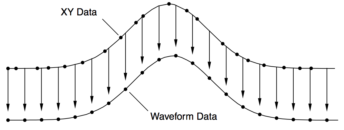
The diagram below shows how the XY pair defining the upper curve is interpolated to compute the uniformly-spaced waveform defining the lower curve. Each arrow indicates an interpolated waveform value:

Igor provides three tools for doing this interpolation: The XY Pair to Waveform panel, the built-in interp function and the Interpolate2 operation. To illustrate these tools we need some sample XY data. The following commands make sample data and display it in a graph:

Make/N=100 xData = .01*x + gnoise(.01)
Make/N=100 yData = 1.5 + 5*exp(-((xData-.5)/.1)^2)
Display yData vs xData

This creates a Gaussian shape. The x wave in our XY pair has some noise in it so the data is not uniformly spaced in the X dimension.

The x data goes roughly from 0 to 1.0 but, because our x data has some noise, it may not be monotonic. This means that, as we go from one point to the next, the x data usually increases but at some points may decrease. We can fix this by sorting the data.

Sort xData, xData, yData

This command uses the xData wave as the sort key and sorts both xData and yData so that xData always increases as we go from one point to the next.

Using the XY Pair to Waveform Panel

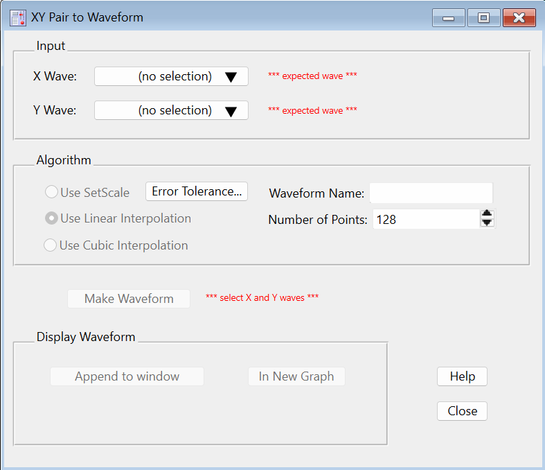
The XY Pair to Waveform panel creates a waveform from XY data using the SetScale or Interpolate2 operations, based on an automatic analysis of the X wave's data.

The required steps are:

1. Select XY Pair to Waveform from Igor's Data→Packages submenu. The panel is displayed:

   

2. Select the X and Y waves (xData and yData) in the popup menus. When this example's xData wave is analyzed it is found to be "not regularly spaced (slope error avg= 0.52...)", which means that SetScale is not appropriate for converting yData into a waveform.

3. Use Interpolate is selected here, so you need a waveform name for the output. Enter any valid wave name.

4. Set the number of output points. Using a number roughly the same as length of the input waves is a good first attempt. You can choose a larger number later if the fidelity to the original is insufficient. A good number depends on how uneven the X values are - use more points for more unevenness.

5. Click Make Waveform.

6. To compare the XY representation of the data with the waveform representation, append the waveform to a graph displaying the XY pair. Make that graph the top graph, then click the Append to <Name of Graph> button.

7. You can revise the Number of Points and click Make Waveform to overwrite the previously created waveform in-place.

Using the Interp Function

We can use the interp function to create a waveform version of our Gaussian. The required steps are:

1. Make a new wave to contain the waveform representation.

2. Use the SetScale operation to define the range of X values in the waveform.

3. Use the interp function to set the data values of the waveform based on the XY data.

Here are the commands:

Duplicate yData, wData
SetScale/I x 0, 1, wData
wData = interp(x, xData, yData)

To compare the waveform representation to the XY representation, we append the waveform to the graph.

AppendToGraph wData

Let's take a closer look at what these commands are doing.

First, we cloned yData and created a new wave, wData. Since we used Duplicate, wData will have the same number of points as yData. We could have made a waveform with a different number of points. To do this, we would use the Make operation instead of Duplicate.

The SetScale operation sets the X scaling of the wData waveform. In this example, we are setting the X values of wData to go from 0 up to and including 1.0. This means that our waveform representation will contain 100 values at uniform intervals in the X dimension from 0 to 1.0.

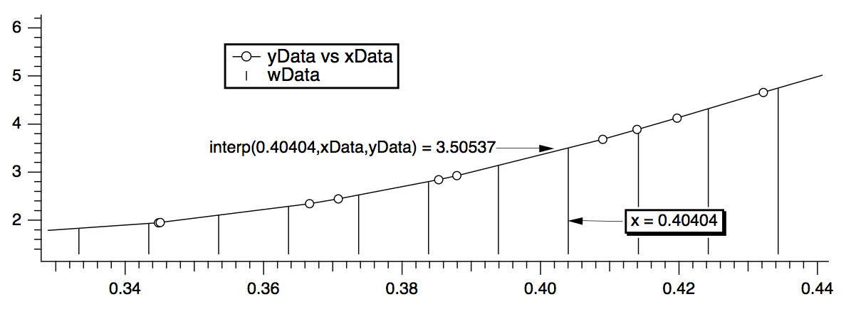
The last step uses a waveform assignment to set the data values of wData. This assignment evaluates the right-hand expression once for each point in wData. For each evaluation, x takes on a different value from 0 to 1.0. The interp function returns the value of the curve yData versus xData at x. For instance, x=.40404 (point number 40 of wData) falls between two points in the XY curve. The interp function linearly interpolates between those values to estimate a data value of 3.50537:

We can wrap these calculations up into an Igor procedure that can create a waveform version of any XY pair.

Function XYToWave1(xWave, yWave, wWaveName, numPoints)
	Wave/D xWave         // X wave in the XY pair
	Wave/D yWave         // Y wave in the XY pair
	String wWaveName     // Name to use for new waveform wave
	Variable numPoints   // Number of points for waveform

	Make/O/N=(numPoints) $wWaveName  // Make waveform.
	Wave wWave= $wWaveName
	WaveStats/Q xWave                // Find range of x coords
	SetScale/I x V_min, V_max, wWave // Set X scaling for wave
	wWave = interp(x, xWave, yWave)  // Do the interpolation
End

This function uses the WaveStats operation to find the X range of the XY pair. WaveStats creates the variables V_min and V_max (among others). See Accessing Variables Used by Igor Operations for details.

The function makes the assumption that the input waves are already sorted. We left the sort step out because the sorting would be a side-effect and we prefer that procedures not have nonobvious side effects.

To use the WaveMetrics-supplied XYToWave1 function, include the "XY Pair To Waveform" procedure file. See The Include Statement for instructions on including a procedure file.

If you have blanks (NaNs) in your input data, the interp function will give you blanks in your output waveform as well. The Interpolate2 operation, discussed in the next section, interpolates across gaps in data and does not produce blanks in the output.

Using the Interpolate2 Operation

The Interpolate2 operation provides not only linear but also cubic and smoothing spline interpolation. Furthermore, it does not require the input to be sorted and can automatically make the destination waveform and set its X scaling. It also has a dialog that makes it easy to use interactively.

To use it on our sample XY data, choose Analysis→Interpolate and set up the dialog as shown below.

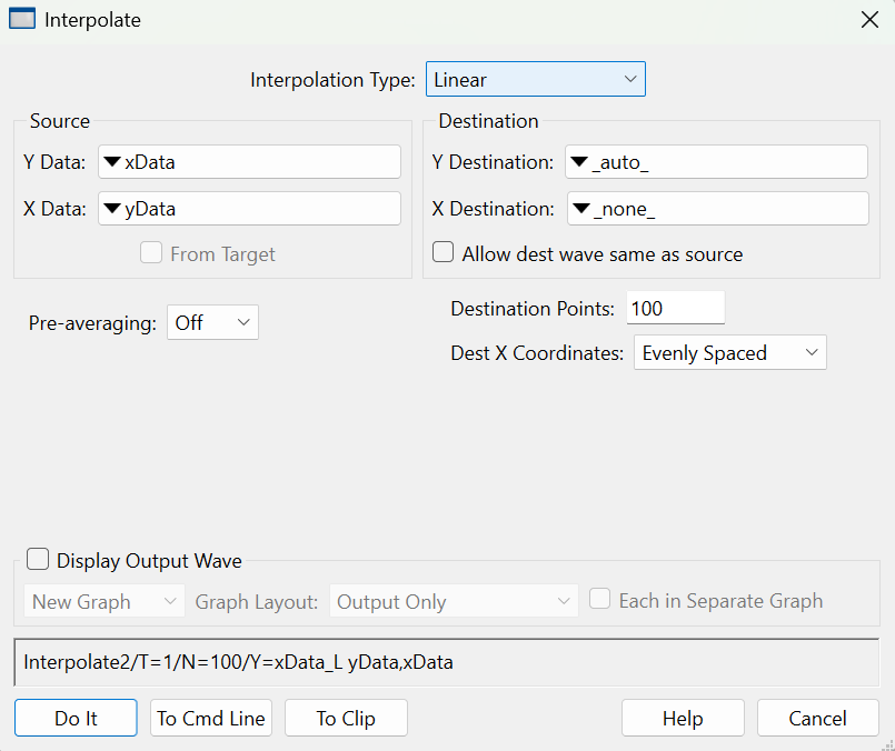
Choosing "_auto_" for Y Destination auto-names the destination wave by appending "_L" to the name of the input "Y data" wave. Choosing "_none_" as the "X destination" tells Interpolate that we want to make a waveform from the input XY pair rather than making a new XY pair.

Here is a rewrite of the XYToWave1 function that uses the Interpolate2 operation rather than the interp function.

Function XYToWave2(xWave, yWave, wWaveName, numPoints)
	Wave xWave           // X wave in the XY pair
	Wave yWave           // Y wave in the XY pair
	String wWaveName     // Name to use for new waveform wave
	Variable numPoints   // Number of points for waveform

	Interpolate2/T=1/N=(numPoints)/Y=$wWaveName xWave, yWave
End

Blanks in the input data are ignored.

For details on Interpolate2, see The Interpolate2 Operation.

Dealing with Missing Values

A missing value is represented in Igor by the value NaN which means "Not a Number". A missing value is also called a "blank", because it appears as a blank cell in a table.

When a NaN is combined arithmetically with any value, the result is NaN. To see this, try the following command:

Print 3+NaN, NaN/5, sin(NaN)

By definition, a NaN is not equal to anything. Consequently, the condition in this statement:

if (myValue == NaN)

is always false.

The workaround is to use the NumType function:

if (NumType(myValue) == 2) 	// Is it a NaN?

See also NaNs, INFs and Missing Values for more about how NaN values.

Some routines in Igor deal with missing values by ignoring them. CurveFit is one example. Others may produce unexpected results in the presence of missing values. Examples are the FFT operation and the area and mean functions.

Here are some strategies for dealing with missing values.

Replace the Missing Values With Another Value

You can replace NaNs in a wave with this statement:

wave0 = NumType(wave0)==2 ? 0:wave0 // Replace NaNs with zero

If you're not familiar with the :? operator, see ? :.

For multi-dimensional waves you can replace NaNs using MatrixOp. For example:

Make/O/N=(3,3) matNaNTest = p + 10*q
Edit matNaNTest
matNaNTest[0][0] = NaN; matNaNTest[1][1] = NaN; matNaNTest[2][2] = NaN
MatrixOp/O matNaNTest=ReplaceNaNs(matNaNTest,0)	// Replace NaNs with 0

Remove the Missing Values

For 1D waves you can remove NaNs using WaveTransform zapNaNs. For example:

Make/N=5 NaNTest = p
Edit NaNTest
NaNTest[1] = NaN; NaNTest[4] = NaN
WaveTransform zapNaNs, NaNTest

There is no built-in operation to remove NaNs from an XY pair if the NaN appears in either the X or Y wave. You can do this, however, using the RemoveNaNsXY procedure in the "Remove Points" WaveMetrics procedure file which you can access through Help→Windows→WM Procedures Index.

There is no operation to remove NaNs from multi-dimensional waves as this would require removing the entire row and entire column where each NaN appeared.

Work Around Gaps in Data

Many analysis routines can work on a subrange of data. In many cases you can just avoid the regions of data that contain missing values. In other cases you can extract a subset of your data, work with it and then perhaps put the modified data back into the original wave.

Here is an example of extract-modify-replace (even though Smooth properly accounts for NaNs):

Make/N=100 data1= sin(P/8)+gnoise(.05); data1[50]= NaN
Display data1
Duplicate/R=[0,49] data1,tmpdata1	// start work on first set
Smooth 5,tmpdata1
data1[0,49]= tmpdata1[P]				// put modified data back
Duplicate/O/R=[51,] data1,tmpdata1	// start work on 2nd set
Smooth 5,tmpdata1
data1[51,]= tmpdata1[P-51]
KillWaves tmpdata1

Replace Missing Data with Interpolated Values

You can replace NaN data values prior to performing operations that do not take kindly to NaNs by replacing them with smoothed or interpolated values using Smooth, Loess, or The Interpolate2 Operation.

Replace Missing Data using the Interpolate2 Operation

By using the same number of points for the destination as you have source points, you can replace NaNs without modifying the other data.

If you have waveform data, simply duplicate your data and perform linear interpolation using the same number of points as your data. For example, assuming 100 data points:

Duplicate data1,data1a
Interpolate/T=1/N=100/Y=data1a data1

If you have XY data, the Interpolate2 operation has the ability to include the input x values in the output X wave. For example:

Duplicate data1, yData1, xData1
xData1 = x
Display yData1 vs xData1
Interpolate2/T=1/N=100/I/Y=yData1a/X=xData1a xData1,yData1

If, after performing an operation on your data, you wish to put the modified data back in the source wave while maintaining the original missing values you can use a wave assignment similar to this:

yData1 = (numtype(yData1) == 0) ? yData1 : yData1a

This technique can also be applied using interpolated results generated by the Loess and Smooth operations.

Replace Missing Data using Median Smoothing

You can use the Smooth dialog to replace each NaN with the median of surrounding values.

Select the Median smoothing algorithm, select "NaNs" from the Replace popup, and choose "Median" for the "with:" radio button. Enter the number of surrounding points used to compute the median (an odd number is best).

You can choose to overwrite the NaNs or create a new waveform with the result. The Smooth dialog produces commands like this:

Duplicate/O data1,data1_smth;DelayUpdate
Smooth/M=(NaN) 5, data1_smth

Interpolation

Igor Pro has a number of interpolation tools that are designed for different applications. We summarize these in the table below.

Data	Operation/Function	Interpolation Method
1D waves	Wave assignment, e.g., val=wave(x)	Linear
1D waves	Smooth	Running median, average, binomial, Savitsky-Golay
1D XY waves	interp	Linear
1D single or XY waves	The Interpolate2 Operation	Linear, cubic spline, smoothing spline
1D or 2D single or XY	Loess	Locally-weighted regression
Triplet XYZ waves	ImageInterpolate	Voronoi
1D X, Y, Z waves	Data→Packages→XYZ to Matrix	Voronoi
1D X, Y, Z waves	Loess	Locally-weighted regression
2D waves	ImageInterpolate	Bilinear, splines, Kriging, Voronoi
2D waves	Interp2D	Bilinear
2D waves	SphericalInterpolate	Voronoi
3D waves	Interp3d	extractSurface, Trilinear
	Interp3DPath	extractSurface, Trilinear
	ImageTransform	extractSurface, Trilinear
3D scatter data	Interpolate3D	Barycentric
4D waves	Interp4D	4D Linear
	Interp4dPath	4D Linear

All the interpolation methods in this table consist of two common steps. The first step involves the identification of data points that are nearest to the interpolation location and the second step is the computation of the interpolated value using the neighboring values and their relative proximity. You can find the specific details in the documentation of the individual operation or function.

Interpolation Demo

Open Smooth Curve Through Noise Demo

The Interpolate2 Operation

The Interpolate2 operation performs linear, cubic spline and smoothing cubic spline interpolation on 1D waveform and XY data. The cubic spline interpolation is based on a routine in "Numerical Recipes in C". The smoothing spline is based on "Smoothing by Spline Functions", Christian H. Reinsch, Numerische Mathematic 10, 177-183 (1967).

Prior to Igor 7, Interpolate2 was implemented as part of the Interpolate XOP. It is now built-in.

The Interpolate XOP also implemented an older operation named Interpolate which used slightly different syntax. If you are using the Interpolate operation, we recommend that you convert to using Interpolate2.

The main use for linear interpolation is to convert an XY pair of waves into a single wave containing Y values at evenly spaced X values so that you can use Igor operations, like FFT, which require evenly spaced data.

Cubic spline interpolation is most useful for putting a pleasingly smooth curve through arbitrary XY data. The resulting curve may contain features that have nothing to do with the original data so you should be wary of using the cubic spline for analytic rather than esthetic purposes.

Both linear and cubic spline interpolation are constrained to put the output curve through all of the input points and thus work best with a small number of input points. The smoothing spline does not have this constraint and thus works well with large, noisy data sets.

The Interpolate2 operation has a feature called "pre-averaging" which can be used when you have a large number of input points. Pre-averaging was added to Interpolate2 as a way to put a cubic spline through a large, noisy data set before it supported the smoothing spline. We now recommend that you try the smoothing spline instead of pre-averaging.

The Smooth Curve Through Noise example experiment illustrates spline interpolation.

Open Smooth Curve Through Noise Demo

Spline Interpolation Example

Before going into a complete discussion of Interpolate2, let's look at a simple example first.

note

You can execute the commands in this example by selecting them and pressing control-return or control-enter.

First, make some sample XY data using the following commands:

Make/N=10 xData, yData                       // Make source data
xData = p; yData = 3 + 4*xData + gnoise(2)   // Create sample data
Display yData vs xData                       // Make a graph
Modify mode=2, lsize=3                       // Display source data as dots

Now, choose Analysis→Interpolate to invoke the Interpolate dialog.

Set Interpolation Type to Cubic Spline.

Choose yData from the Y Data pop-up menu.

Choose xData from the X Data pop-up menu.

Choose _auto_ from the Y Destination pop-up menu.

Choose _none_ from the X Destination pop-up menu.

Enter 200 in the Destination Points box.

Choose Off from the Pre-averaging pop-up menu.

Choose Evenly Spaced from the Dest X Coords pop-up menu.

Click Natural in the End Points section.

Notice that the dialog has generated the following command:

Interpolate2/T=2/N=200/E=2/Y=yData_CS xData, yData

This says that Interpolate2 will use yData as the Y source wave, xData as the X source wave and that it will create yData_CS as the destination wave. _CS means "cubic spline".

Click the Do It button to do the interpolation.

Now add the yData_CS destination wave to the graph using the command:

AppendToGraph yData_CS; Modify rgb(yData_CS)=(0,0,65535)

Now let's try this with a larger number of input data points. Execute:

Redimension/N=500 xData, yData
xData = p/50; yData = 10*sin(xData) + gnoise(1.0)	// Create sample data
Modify lsize(yData)=1			// Smaller dots

Now choose Analysis→Interpolate to invoke the Interpolate dialog. All the settings should be as you left them from the preceding exercise. Click the Do It button.

Notice that the resulting cubic spline attempts to go through all of the input data points. This is usually not what we want.

Now, choose Analysis→Interpolate again and make the following changes:

Choose Smoothing Spline from the Interpolation Type pop-up menu. Notice the command generated now references a wave named yData_SS. This will be the output wave.

Enter 1.0 for the smoothing factor. This is usually a good value to start from.

In the Standard Deviation section, click the Constant radio button and enter 1.0 as the standard deviation value. 1.0 is correct because we know that our data has noise with a standard deviation of 1.0, as a result of the "gnoise(1.0)" term above.

Click the Do It button to do the interpolation. Append the yData_SS destination wave to the graph using the command:

AppendToGraph yData_SS; Modify rgb(yData_SS)=(0,0,0)

Notice that the smoothing spline adds a pleasing curve through the large, noisy data set. If necessary, enlarge the graph window so you can see this.

You can tweak the smoothing spline using either the smoothing factor parameter or the standard deviation parameter. If you are unsure of the standard deviation of the noise, leave the smoothing factor set to 1.0 and try different standard deviation values. It is usually not too hard to find a reasonable value.

The Interpolate Dialog

Choosing Analysis→Interpolate summons the Interpolate dialog from which you can choose the desired type of interpolation, the source wave or waves, the destination wave or waves, and the number of points in the destination waves. This dialog generates an Interpolate2 command which you can execute, copy to the clipboard or copy to the command line.

From the Interpolation Type pop-up menu, choose Linear or Cubic Spline or Smoothing Spline. Cubic spline is good for a small input data set. Smoothing spline is good for a large, noisy input data set.

If you choose Cubic Spline, a Pre-averaging pop-up menu appear. The pre-averaging feature is largely no longer needed and is not recommended. Use the smoothing spline instead of the cubic spline with pre-averaging.

If you choose smoothing spline, a Smoothing Factor item and Standard Deviant controls appear. Usually it is best to set the smoothing factor to 1.0 and use the constant mode for setting the standard deviation. You then need to enter an estimate for the standard deviation of the noise in your Y data. Then try different values for the standard deviation until you get a satisfactory smooth spline through your data. See Smoothing Spline Parameters for further details.

From the Y Data and X Data pop-up menus, choose the source waves that define the data through which you want to interpolate. If you choose a wave from the X Data pop-up, Interpolate2 uses the XY curve defined by the contents of the Y data wave versus the contents of the X data wave as the source data. If you choose _calculated_ from the X Data pop-up, it uses the X and Y values of the Y data wave as the source data.

If you click the From Target checkbox, the source and destination pop-up menus show only waves in the target graph or table.

The X and Y data waves must have the same number of points. They do not need to have the same data type.

The X and Y source data does not need to be sorted before using Interpolate2. If necessary, Interpolate2 sorts a copy of the input data before doing the interpolation.

NaNs (missing values) and INFs (infinite values) in the source data are ignored. Any point whose X or Y value is NaN or INF is treated as if it did not exist.

Enter the number of points you want in the destination waves in the Destination Points box. 200 points is usually good.

From the Y Destination and X Destination pop-up menus, choose the waves to contain the result of the interpolation. For most cases, choose _auto_ for the Y destination wave and _none_ for the X destination wave. This gives you an output waveform. Other options, useful for less common applications, are described in the following paragraphs.

If you choose _auto_ from the Y Destination pop-up, Interpolate2 puts the Y output data into a wave whose name is derived by adding a suffix to the name of the Y data wave. The suffix is "_L" for linear interpolation, "_CS" for cubic spline interpolation and "_SS" for smoothing spline interpolation. For example, if the Y data wave is called "yData", then the default Y destination wave will be called "yData_L", "yData_CS" or "yData_SS".

If you choose _none_ for the X destination wave, Interpolate2 puts the Y output data in the Y destination wave and sets the X scaling of the Y destination wave to represent the X output data.

If you choose _auto_ from the X Destination pop-up, Interpolate2 puts the X output data into a wave whose name is derived by adding the appropriate suffix to the name of the X data wave. If the X data wave is "xData" then the X destination wave will be "xData_L", "xData_CS" or "xData_SS". If there is no X data wave then the X destination wave name is derived by adding the letter "x" to the name of the Y destination wave. For example, if the Y destination is "yData_CS" then the X destination wave will be "yData_CSx".

For both the X and the Y destination waves, if the wave already exists, Interpolate2 overwrites it. If it does not already exist, Interpolate2 creates it.

The destination waves will be double-precision unless they already exist when Interpolate2 is invoked. In this case, Interpolate2 leaves single-precision destination waves as single-precision. For any other precision, Interpolate2 changes the destination wave to double-precision.

The Dest X Coords pop-up menu gives you control over the X locations at which the interpolation is done. Usually you should choose Evenly Spaced. This generates interpolated values at even intervals over the range of X input values.

The Evenly Spaced Plus Input X Coords setting is the same as Evenly Spaced except that Interpolate2 makes sure that the output X values include all of the input X values. This is usually not necessary. This mode is not available if you choose _none_ for your X destination wave.

The Log Spaced setting makes the output evenly spaced on a log axis. This mode ignores any non-positive values in your input X data. It is not available if you choose _none_ for your X destination wave. See Interpolating Exponential Data for an alternative.

The From Dest Wave setting takes the output X values from the X coordinates of the destination wave. The Destination Points setting is ignored. You could use this, for example, to get a spline through a subset of your input data. You must create your destination waves before doing the interpolation for this mode. If your destination is a waveform, use the SetScale operation to define the X values of the waveform. Interpolate2 will calculate its output at these X values. If your destination is an XY pair, set the values of the X destination wave. Interpolate2 will create a sorted version of these values and will then calculate its output at these values. If the X destination wave was originally reverse-sorted, Interpolate2 will reverse the output.

The End Points radio buttons apply only to the cubic spline. They control the destination waves in the first and last intervals of the source wave. Natural forces the second derivative of the spline to zero at the first and last points of the destination waves. Match 1st Derivative forces the slope of the spline to match the straight lines drawn between the first and second input points, and between the last and next-to-last input points. In most cases it doesn't much matter which of these alternatives you use.

Interpolating Exponential Data

It is common to plot data that spans orders of magnitude, such as data arising from exponential processes, versus log axes. To create an interpolated data set from such data, it is often best to interpolate the log of the original data rather than the original data itself.

The Interpolate2 Log Demo experiment demonstrates how to do such interpolation. Here is a snippet from that demo experiment:

Function DoLogYInterpolate2(xInput, yInput, numOutputPoints, xOutput, yOutput)
	Wave xInput, yInput
	int numOutputPoints
	Wave& xOutput			// Output wave reference
	Wave& yOutput			// Output wave reference
	
	// Create log(yInput) to use in interpolation
	Duplicate/FREE yInput, logYInput		// Free wave is automatically killed when function exits
	logYInput = log(yInput)
	
	String xOutName = NameOfWave(xInput) + "_interp"
	String yOutName = NameOfWave(yInput) + "_interp"
	Interpolate2 /T=1 /I=0 /N=(numOutputPoints) /X=$xOutName /Y=$yOutName xInput, logYInput
	
	WAVE xOutput = $xOutName
	WAVE yOutput = $yOutName
	
	// yOutput was set based on log(yInput). Transform it back to original scale.
	yOutput = 10^yOutput
End

Open Interpolate2 Log Demo

Smoothing Spline Algorithm

The smoothing spline algorithm is based on "Smoothing by Spline Functions", Christian H. Reinsch, Numerische Mathematik 10. It minimizes

$$\displaystyle \int_{x_{0}}^{x_{n}} g^{\prime \prime}(x)^{2} d x,$$

among all functions g(x) such that

$$\displaystyle \sum_{i=0}^{n}\left(\frac{g\left(x_{i}\right)-y_{i}}{\sigma_{i}}\right)^{2} \leq S,$$

where g(x_i) is the value of the smooth spline at a given point, y_i is the Y data at that point, σ_i is the standard deviation of that point, and S is the smoothing factor.

Smoothing Spline Parameters

The smoothing spline operation requires a standard deviation parameter and a smoothing factor parameter. The standard deviation parameter should be a good estimate of the standard deviation of the noise in your Y data. The smoothing factor should nominally be close to 1.0, assuming that you have an accurate standard deviation estimate.

Using the Standard Deviation section of the Interpolate dialog, you can choose one of three options for the standard deviation parameter: None, Constant, From Wave.

If you choose None, Interpolate2 uses an arbitrary standard deviation estimate of 0.05 times the amplitude of your Y data. You can then play with the smoothing factor parameter until you get a pleasing smooth spline. Start with a smoothing factor of 1.0. This method is not recommended.

If you choose Constant, you can then enter your estimate for the standard deviation of the noise and Interpolate2 uses this value as the standard deviation of each point in your Y data. If your estimate is good, then a smoothing factor around 1.0 will give you a nice smooth curve through your data. If your initial attempt is not quite right, you should leave the smoothing factor at 1.0 and try another estimate for the standard deviation. For most types of data, this is the preferred method.

If you choose From Wave then Interpolate2 expects that each point in the specified wave contains the estimated standard deviation for the corresponding point in the Y data. You should use this method if you have an appropriate wave.

Interpolate2's Pre-averaging Feature

A linear or cubic spline interpolation goes through all of the input data points. If you have a large, noisy data set, this is probably not what you want. Instead, use the smoothing spline.

Before Interpolate2 had a smoothing spline, we recommended that you use the cubic spline to interpolate through a decimated version of your input data. The pre-averaging feature was designed to make this easy.

Because Interpolate2 now supports the smoothing spline, the pre-averaging feature is no longer necessary. However, we still support it for backward compatibility.

When you turn pre-averaging on, Interpolate2 creates a temporary copy of your input data and reduces it by decimation to a smaller number of points, called nodes. Interpolate2 then usually adds nodes at the very start and very end of the data. Finally, it does an interpolation through these nodes.

Identical Or Nearly Identical X Values

This section discusses a degenerate case that is of no concern to most users.

Input data that contains two points with identical X values can cause interpolation algorithms to produce unexpected results. To avoid this, if Interpolate2 encounters two or more input data points with nearly identical X values, it averages them into one value before doing the interpolation. This behavior is separate from the pre-averaging feature. This is done for the cubic and smoothing splines except when the Dest X Coords mode is is Log Spaced or From Dest Wave. It is not done for linear interpolation.

Two points are considered nearly identical in X if the difference in X between them (dx) is less than 0.01 times the nominal dx. The nominal dx is computed as the X span of the input data divided by the number of input data points.

Destination X Coordinates from Destination Wave

This mode, which we call "X From Dest" mode for short, takes effect if you choose From Dest Wave from the Dest X Coords pop-up menu in the Interpolate dialog or use the Interpolate2 /I=3 flag. In this mode the number of output points is determined by the destination wave and the /N flag is ignored.

In X From Dest mode, the points at which the interpolation is done are determined by the destination wave. The destination may be a waveform, in which case the interpolation is done at its X values. Alternatively the destination may be an XY pair in which case the interpolation is done at the data values stored in the X destination wave.

Here is an example using a waveform as the destination:

Make /O /N=20 wave0		// Generate source data
SetScale x 0, 2*PI, wave0
wave0 = sin(x) + gnoise(.1)
Display wave0
ModifyGraph mode=3
Make /O /N=1000 dest0		// Generate dest waveform
SetScale x 0, 2*PI, dest0
AppendToGraph dest0
ModifyGraph rgb(dest0)=(0,0,65535)
Interpolate2 /T=2 /I=3 /Y=dest0 wave0			// Do cubic spline interpolation

If your destination is an XY pair, Interpolate2 creates a sorted version of these values and then calculates its output at the X destination wave's values. If the X destination wave was originally reverse-sorted, as determined by examining its first and last values, Interpolate2 reverses the output after doing the interpolation to restore the original ordering.

In X From Dest mode with an XY pair as the destination, the X wave may contain NaNs. In this case, Interpolate2 creates an internal copy of the XY pair, removes the points where the X destination is NaN, does the interpolation, and copies the results to the destination XY pair. During this last step, Interpolate2 restores the NaNs to their original locations in the X destination wave. Here is an example of an XY destination with a NaN in the X destination wave:

Make/O xData={1,2,3,4,5}, yData={1,2,3,4,5}	// Generate source data
Display yData vs xData
Make/O xDest={1,2,NaN,4,5}, yDest={0,0,0,0,0}	// Generate dest XY pair
ModifyGraph mode=3,marker=19
AppendToGraph yDest vs xDest
ModifyGraph rgb(yDest)=(0,0,65535)
Interpolate2 /T=1 /I=3 /Y=yDest /X=xDest xData, yData	// Do linear interpolation

Differentiation and Integration

The Differentiate and Integrate operations provide a number of algorithms for operation on one-dimensional waveform and XY data. These operations can either replace the original data or create a new wave with the results. The easiest way to use these operations is via dialogs available from the Analysis menu.

For most applications, trapezoidal integration and central differences differentiation are appropriate methods. However, when operating on XY data, the different algorithms have different requirements for the number of points in the X wave. If your X wave does not show up in the dialog, try choosing a different algorithm or click the help button to see what the requirements are.

When operating on waveform data, X scaling is taken into account; you can turn this off using the /P flag. You can use the SetScale operation to define the X scaling of your Y data wave.

Although these operations work along just one dimension, they can be targeted to operate along rows or columns of a matrix (or even higher dimensions) using the /DIM flag.

The Integrate operation replaces or creates a wave with the numerical integral. For finding the area under a curve, see Areas and Means.

Areas and Means

You can compute the area and mean value of a wave in several ways using Igor.

Perhaps the simplest way to compute a mean value is with the Wave Stats dialog in the Statistics menu. You select the wave, type in the X range (or use the current cursor positions), click Do It, and Igor prints several statistical results to the history area. Among them is V_avg, which is the average, or mean value. This is the same value that is returned by Igor's mean function, which is faster because it doesn't compute any other statistics. The mean function returns NaN if any data within the specified range is NaN. The WaveStats operation, on the other hand, ignores such missing values.

WaveStats and the mean function use the same method for computing the mean: find the waveform values within the given X range, sum them together, and divide by the number of values. The X range serves only to select the values to combine. The range is rounded to the nearest point numbers.

If you consider your data to describe discrete values, such as a count of events, then you should use either WaveStats or the mean function to compute the average value. You can most easily compute the total number of events, which is an area of sorts, using the sum function. It can also be done easily by multiplying the WaveStats outputs V_avg and V_npnts.

If your data is a sampled representation of a continuous process such as a sampled audio signal, you should use the faverage function to compute the mean, and the area function to compute the area. These two functions use the same linear interpolation scheme as does trapezoidal integration to estimate the waveform values between data points. The X range is not rounded to the nearest point. Partial X intervals are included in the calculation through this linear interpolation.

The diagram below shows the calculations each function performs for the data shown. The two values 43 and 92.2 are linear interpolation estimates. The diagram compares the area, faverage, and mean functions over the interval (12.75,13.32).

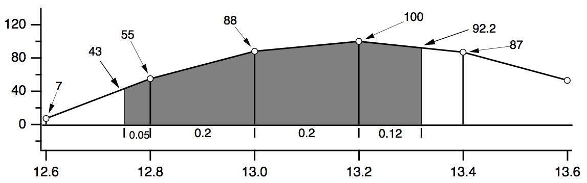
	WaveStats/R=(12.75,13.32) wave
						V_avg = (55+88+100+87)/4 = 82.5

 	mean(wave,12.75,13.32)
						= (55+88+100+87)/4 = 82.5

	area(wave,12.75,13.32) =
						0.05·(43+55)/2		// first trapezoid
					  + 0.20·(55+88)/2		// second trapezoid
					  + 0.20·(88+100)/2		// third trapezoid
					  + 0.12·(100+92.2)/2	// fourth trapezoid
						= 47.082

	faverage(wave,12.75,13.32)	= area(wave,12.75,13.32) / (13.32-12.75)
						= 47.082/0.57 = 82.6

Note that only the area function is affected by the X scaling of the wave. faverage eliminates the effect of X scaling by dividing the area by the same X range that area multiplied by.

One problem with these functions is that they cannot be used if the given range of data has missing values (NaNs). See Dealing with Missing Values for details.

X Ranges and the Mean, faverage, and area Functions

The X range input for the mean, faverage and area functions are optional. Thus, to include the entire wave you don't have to specify the range:

Make/N=10 wave=2; Edit wave.xy            // X ranges from 0 to 9
Print area(wave)                          // entire X range, and no more
18

Sometimes, in programming, it is not convenient to determine whether a range is beyond the ends of a wave. Fortunately, these functions also accept X ranges that go beyond the ends of the wave.

Print area(wave, 0, 9)                    // entire X range, and no more
18

You can use expressions that evaluate to a range beyond the ends of the wave:

Print leftx(wave),rightx(wave)
0  10
Print area(wave,leftx(wave),rightx(wave)) // entire X range, and more
18

or even an X range of ±∞:

Print area(wave, -Inf, Inf)               // entire X range of the universe
18

Finding the Mean of Segments of a Wave

Under Analysis Programming is a function that finds the mean of segments of a wave where you specify the length of the segments. It creates a new wave to contain the means for each segment.

Area for XY Data

To compute the area of a region of data contained in an XY pair of waves, use the areaXY function. There is also an XY version of the faverage function; see faverageXY .

In addition you can use the AreaXYBetweenCursors WaveMetrics procedure file which contains the AreaXYBetweenCursors and AreaXYBetweenCursorsLessBase procedures. For instructions on loading the procedure file, see WaveMetrics Procedures Folder. Use the Info Panel and Cursors to delimit the X range over which to compute the area. AreaXYBetweenCursorsLessBase removes a simple trapezoidal baseline - the straight line between cursors.

Wave Statistics

The WaveStats operation computes various descriptive statistics relating to a wave and prints them in the history area of the command window. It also stores the statistics in a series of special variables or in a wave so you can access them from a procedure.

The statistics printed and the corresponding special variables are:

V_npnts	Number of points in range excluding points whose value is NaN or INF.
V_numNans	Number of NaNs.
V_numINFs	Number of INFs.
V_avg	Average of data values.
V_sum	Sum of data values.
V_sdev	Standard deviation of data values, $\displaystyle \sigma=\sqrt{\frac{\sum\left(Y_{i}-{V\_avg}\right)^{2}}{{V\_npnts}-1}}$
	"Variance" is V_sdev2.
V_sem	Standard error of the mean $\displaystyle { sem }=\frac{\sigma}{\sqrt{V\_npnts}}$
V_rms	RMS of Y values $\displaystyle =\sqrt{\frac{1}{V\_npnts} \sum Y_{i}^{2}}$
V_adev	Average deviation $\displaystyle =\frac{1}{V\_npnts} \sum_{i=0}^{{V\_npts}-1}\left\|Y_{i}-\bar{Y}\right\|$
V_skew	Skewness $\displaystyle =\frac{1}{V\_npnts} \sum_{i=0}^{V\_npnts-1}\left(\frac{Y_{i}-\bar{Y}}{\sigma}\right)^{3}$
V_kurt	Kurtosis $\displaystyle =\left(\frac{1}{V\_npnts} \sum_{i=0}^{V\_npnts-1}\left(\frac{Y_{i}-\bar{Y}}{\sigma}\right)^{4}\right)-3$
V_minloc	X location of minimum data value.
V_min	Minimum data value.
V_maxloc	X location of maximum data value.
V_max	Maximum data value.
V_minRowLoc	Row containing minimum data value.
V_maxRowLoc	Row containing maximum data value.
V_minColLoc	Column containing minimum data value (2D or higher waves).
V_maxColLoc	Column containing maximum data value (2D or higher waves).
V_minLayerLoc	Layer containing minimum data value (3D or higher waves).
V_maxLayerLoc	Layer containing maximum data value (3D or higher waves).
V_minChunkLoc	Chunk containing minimum data value (4D waves only).
V_maxChunkLoc	Chunk containing maximum data value (4D waves only).
V_startRow	The unscaled index of the first row included in calculating statistics.
V_endRow	The unscaled index of the last row included in calculating statistics.
V_startCol	The unscaled index of the first column included in calculating statistics. Set only when /RMD is used.
V_endCol	The unscaled index of the last column included in calculating statistics. Set only when /RMD is used.
V_startLayer	The unscaled index of the first layer included in calculating statistics. Set only when /RMD is used.
V_endLayer	The unscaled index of the last layer included in calculating statistics. Set only when /RMD is used.
V_startChunk	The unscaled index of the first chunk included in calculating statistics. Set only when /RMD is used.
V_endChunk	The unscaled index of the last chunk included in calculating statistics. Set only when /RMD is used.

To use the WaveStats operation, choose Wave Stats from the Statistics menu.

Igor ignores NaNs and INFs in computing the average, standard deviation, RMS, minimum and maximum. NaNs result from computations that have no defined mathematical meaning. They can also be used to represent missing values. INFs result from mathematical operations that have no finite value.

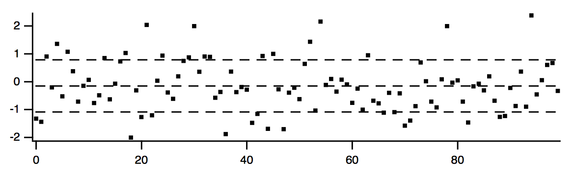
This procedure illustrates the use of WaveStats. It shows the average and standard deviation of a source wave, assumed to be displayed in the top graph. It draws lines to indicate the average and standard deviation.

Function ShowAvgStdDev(source)
	Wave source    // source waveform

	Variable left=leftx(source),right=rightx(source)   // source X range
	WaveStats/Q source
	SetDrawLayer/K ProgFront
	SetDrawEnv xcoord=bottom,ycoord=left,dash= 7
	DrawLine left, V_avg, right, V_avg                 // show average
	SetDrawEnv xcoord=bottom,ycoord=left,dash= 7
	DrawLine left, V_avg+V_sdev, right, V_avg+V_sdev   // show +std dev
	SetDrawEnv xcoord=bottom,ycoord=left,dash= 7
	DrawLine left, V_avg-V_sdev, right, V_avg-V_sdev   // show -std dev
	SetDrawLayer UserFront
End

You could try this function using the following commands.

Make/N=100 wave0 = gnoise(1)
Display wave0; ModifyGraph mode(wave0)=2, lsize(wave0)=3
ShowAvgStdDev(wave0)

When you use WaveStats with a complex wave, you can choose to compute the same statistics as above for the real, imaginary, magnitude and phase of the wave. By default WaveStats only computes the statistics for the real part of the wave. When computing the statistics for other components, the operation stores the results in a multidimensional wave M_WaveStats.

If you are working with large amounts of data and you are concerned about computation speed you might be able to take advantage of the /M flag that limits the calculation to the first order moments.

If you are working with 2D or 3D waves and you want to compute the statistics for a domain of an arbitrary shape you should use the ImageStats operation with an ROI wave.

Histograms

A histogram totals the number of input values that fall within each of a number of value ranges (or "bins") usually of equal extent. For example, a histogram is useful for counting how many data values fall in each range of 0-10, 10-20, 20-30, etc. This calculation is often made to show how students performed on a test:

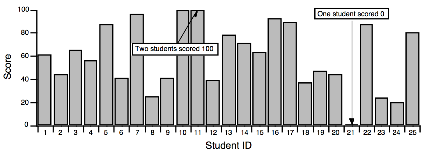
The usual use for a histogram in this case is to figure out how many students fall into certain numerical ranges, usually the ranges associated with grades A, B, C, and D. Suppose the teacher decides to divide the 0-100 range into 4 equal parts, one per grade. The Histogram operation can be used to show how many students get each grade by counting how many students fall in each of the 4 ranges.

We start by creating a wave to hold the histogram output:

Make/O/D/N=4 studentsWithGrade

Next we execute the Histogram command which we generated using the Histogram dialog:

Histogram/B={0,25,4} scores,studentsWithGrade

The /B flag tells Histogram to create four bins, starting from 0 with a bin width of 25. The first bin counts values from 0 up to but not including 25.

The Histogram operation analyzes the source wave (scores), and puts the histogram result into a destination wave (studentsWithGrade).

Let's create a text wave of grades to plot studentsWithGrade versus a grade letter in a category plot:

Make/O/T grades = {"D", "C", "B", "A"}
Display studentsWithGrade vs grades
SetAxis/A/E=1 left

Everything looks good in the category plot. Let's double-check that all the students made it into the bins:

Print sum(studentsWithGrade)
  23

There are two missing students. They are ones who scored 100 on the test. The four bins we defined are actually:

Bin 1: 0 - 24.99999

Bin 2: 25 - 49.99999

Bin 3: 50 - 74.99999

Bin 4: 75 - 99.99999

The problem is that the test scores actually encompass 101 values, not 100. To include the perfect scores in the last bin, we could add a small number such as 0.001 to the bin width:

Bin 1: 0 - 25.00999

Bin 2: 25.001 - 49.00199

Bin 3: 50.002 - 74.00299

Bin 4: 75.003 - 100.0399

The students who scored 25, 50 or 75 would be moved down one grade, however. Perhaps the best solution is to add another bin for perfect scores:

Make/O/T grades= {"D", "C", "B", "A", "A+"}
Histogram/B={0,25,5} scores,studentsWithGrade

For information on plotting a histogram, see Category Plots and Graphing Histogram Results.

This example was intended to point out the care needed when choosing the histogram binning. Our example used "manual binning".

The Histogram operation provides five ways to set binning. They correspond to the Destination Bins radio buttons in the Histogram dialog:

Bin Mode	What It Does
Manual bins	Sets number of points and X scaling of destination wave based on parameters that you explicitly specify.
Auto-set bin range	Sets X scaling of destination wave to cover the range of values in the source wave.
	Does not change the number of points (bins) in the destination wave. Thus, you need to set the number of points yourself before computing the histogram.
	When using the Histogram dialog, if you select Make New Wave or Auto from the Output Wave menu, the dialog must be told how many points the new wave should have. It displays the Number of Bins box to let you specify the number.
Set bins from destination wave	Does not change X scaling or number of points in the destination wave. Thus, you need to set X scaling and number of points yourself before computing the histogram.
	When using the Histogram dialog, the Set from destination wave radio button is only available if you choose Select Existing Wave from the Output Wave menu.
Auto-set bins: 1+log2(N)	Examines the input data and sets the number of bins based on the number of input data points. Sets the bin range the same as if Auto-set bin range were selected.
Auto-set bins: 3.49 * Sdev * N^-1/3	Examines the input data and sets the number of bins based on the number of input data points and the standard deviation of the data. Sets the bin range the same as if Auto-set bin range were selected.
Freedman-Diaconis method	Sets the optimal bin width to binWidth = 2 * IQR * N-1/3 where IQR is the interquartile distance (see StatsQuantiles) and the bins are evenly-distributed between the minimum and maximum values. Added in Igor Pro 7.00.

Histogram Caveats

If you use the "Set bins from destination wave" bin mode, you must create the destination wave, using the Make operation, before computing the histogram. You also must set the X scaling of the destination wave, using the SetScale operation.

The Histogram operation does not distinguish between 1D waves and multidimensional waves. If you use a multidimensional wave as the source wave, it will be analyzed as if the wave were one dimensional. This may still be useful - you will get a histogram showing counts of the data values from the source wave as they fall into bins.

If you would like to perform a histogram of 2D or 3D image data, you may want to use the ImageHistogram operation, which supports specific features that apply to images only.

Graphing Histogram Results

Our example above displayed the histogram results as a category plot because the bins corresponded to text values. Often histogram bins are displayed on a numeric axis. In this case you need to know how Igor displays a histogram result.

For example, this histBins destination wave has 12 points (bins), the first bin starting at -3, and each bin is 0.5 wide. The X scaling is shown in the table:

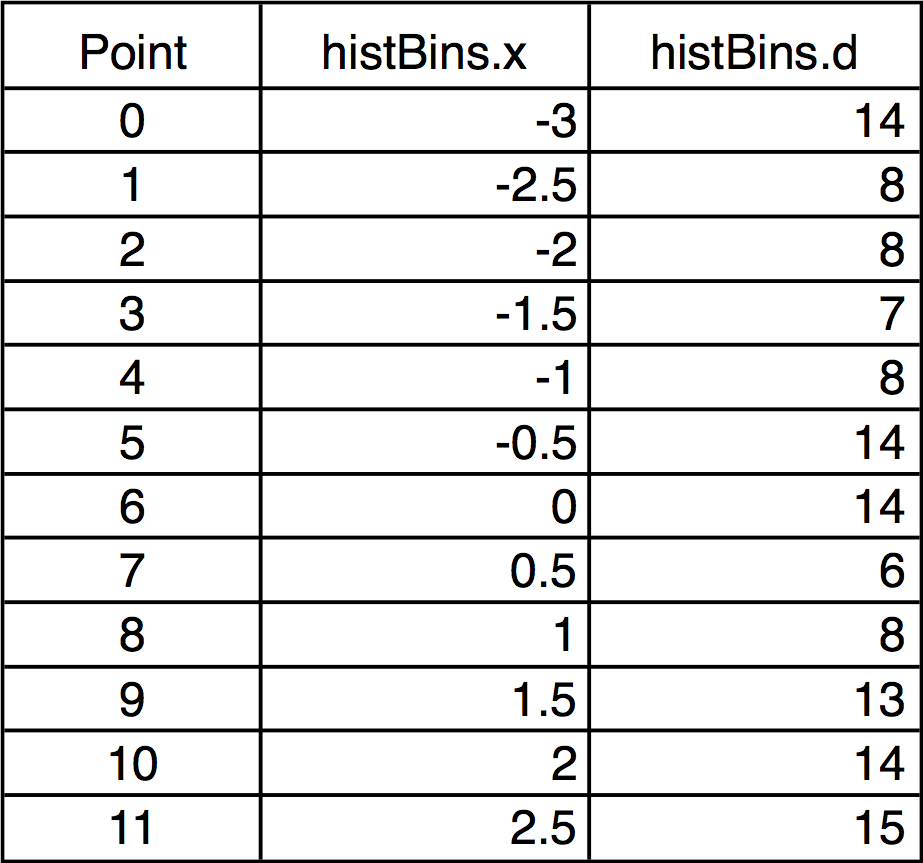
When histBins is graphed in both bars and markers modes, it looks like this:

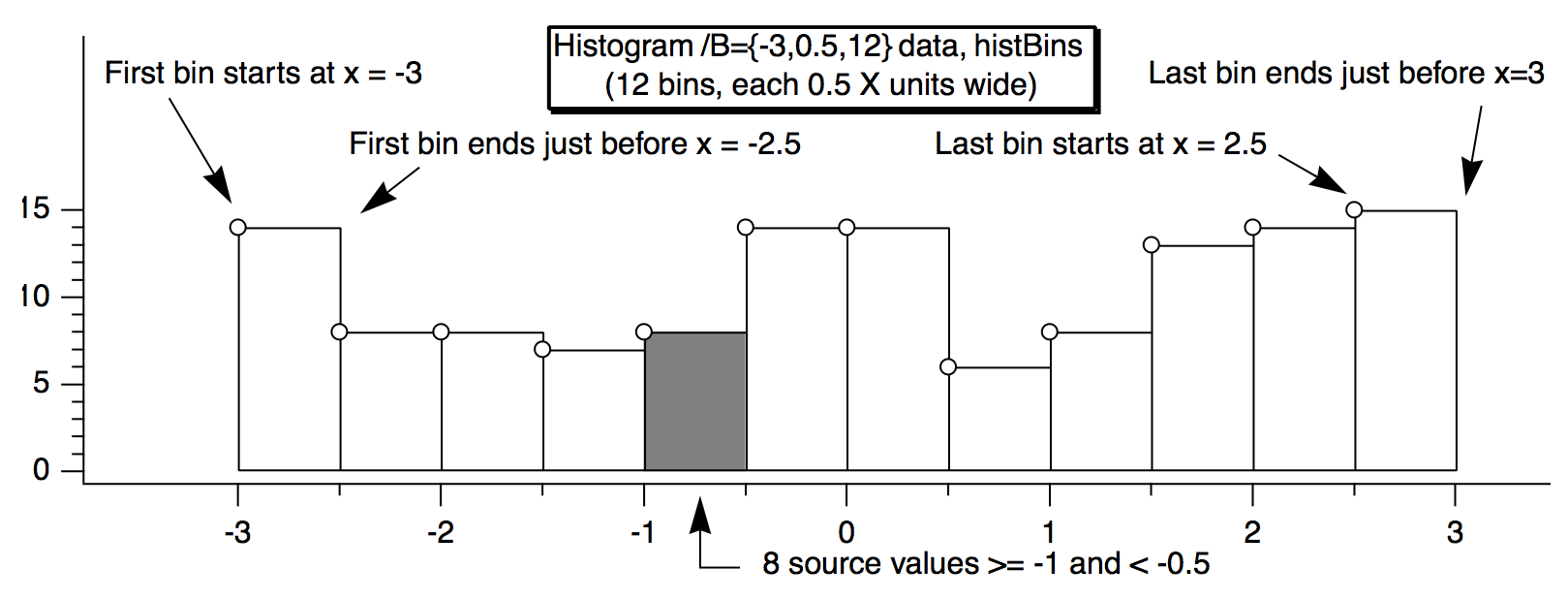
Note that the markers are positioned at the start of the bars. You can offset the marker trace by half the bin width if you want them to appear in the center of the bin.

Alternatively, you can make a second histogram using the Bin-Centered X Values option. In the Histogram dialog, check the Bin-Centered X Values checkbox.

The Histogram Dialog

To use the Histogram operation, choose Histogram from the Analysis menu.

To use the "Manually set bins" or "Set from destination wave" bin modes, you need to decide the range of data values in the source wave that you want the histogram to cover. You can do this visually by graphing the source wave or you can use the WaveStats operation to find the exact minimum and maximum source values.

The dialog requires that you enter the starting bin value and the bin width. If you know the starting bin value and the ending bin value then you need to do some arithmetic to calculate the bin width.

A line of text at the bottom of the Destination Bins box tells you the first and last values, as well as the width and number of bins. This information can help with trial-and-error settings.

If you use the "Manually set bins" or any of the "Auto-set" modes, Igor will set the X units of the destination wave to be the same as the Y units of the source wave.

If you enable the Accumulate checkbox, Histogram does not clear the destination wave but instead adds counts to the existing values in it. Use this to accumulate results from several histograms in one destination. If you want to do this, don't use the "Auto-set bins" option since it makes no sense to change bins in mid-stream. Instead, use the "Set from destination wave" mode. To use the Accumulate option, the destination wave must be double-precision or single-precision and real.

The "Bin-Centered X Values" and "Create Square Root(N) Wave" options are useful for curve fitting to a histogram. If you do not use Bin-Centered X Values, any X position parameter in your fit function will be shifted by half a bin width. The Square Root(N) Wave creates a wave that estimates the standard deviation of the histogram data; this is based on the fact that counting data have a Poisson distribution. The wave created by this option does not try to do anything special with bins having zero counts, so if you use the square root(N) wave to weight a curve fit, these zero-count bins will be excluded from the fit. You may need to replace the zeroes with some appropriate value.

The binning modes were added in Igor Pro. In earlier versions of Igor, the accumulate option had two effects:

• Caused Igor to not clear the destination wave

• Caused Igor to effectively use the "Set bins from destination wave" mode

To maintain backward compatibility, the Histogram operation still behaves this way if the accumulate ("/A") flag is used and no bin ("/B") flag is used. This dialog always generates a bin flag. Thus, the accumulate flag just forces accumulation and has no effect on the binning.

You can use the Histogram operation on multidimensional waves but they are treated as though the data belonged to a single 1D wave. If you are working with 2D or 3D waves you may prefer to use the ImageHistogram operation, which computes the histogram of one layer at a time.

Histogram Example

The following commands illustrate a simple test of the histogram operation.

SetRandomSeed 0.2                               // For reproducible randomness
Make/O/N=10000 noise = gnoise(1)                // Make raw data
Make/O hist                                     // Make destination wave
Histogram/B={-3, (3 - -3)/100, 100} noise, hist // Perform histogram
Display hist; Modify mode(hist)=1

These commands produce the following graph:

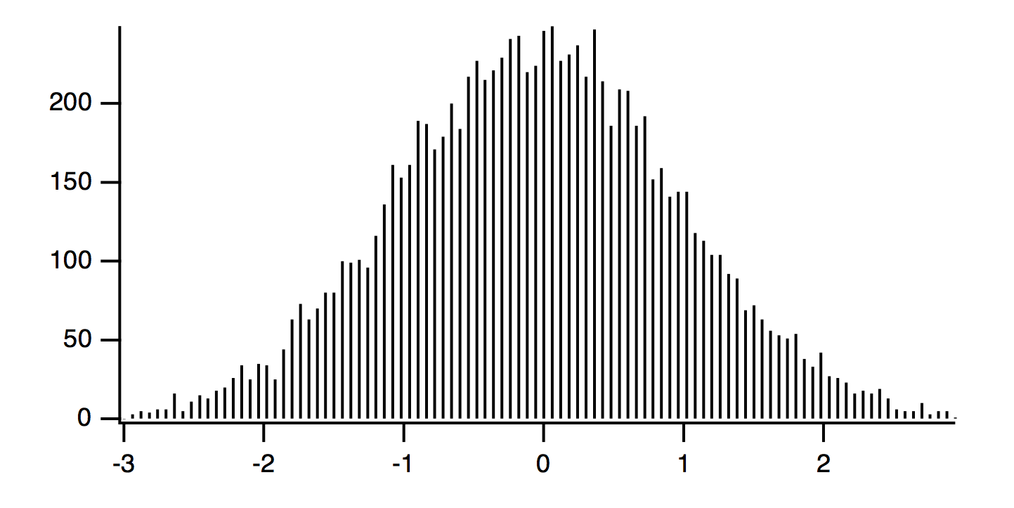
The raw data has 10,000 samples drawn from a Gaussian distribution having standard deviation of 1.0, and mean of zero. The histogram is made with 100 bins with width of 6/100 = 0.06. The amplitude of the histogram is expected to be:

A = (N*dx)/sqrt(2*pi)/sigma = (10000*0.06)/sqrt(2*pi)/1 = 239.365

The X scaling of the wave hist uses the Histogram default of the left side of the bins.

Curve Fitting to a Histogram

Because the values in the source wave are Gaussian deviates generated by the gnoise function, the histogram should have the familiar Gaussian bell-shape. You can estimate the characteristics of the population the samples were taken from by fitting a Gaussian curve to the data. First try fitting a Gaussian curve to the example histogram:

CurveFit gauss hist /D					// Curve fit to histogram

The solution from the curve fit is:

y0    =	-0.85917 ± 2.74
A     =	238.23 ± 3.07
x0    =	-0.047537 ± 0.0113
width =	1.4337 ± 0.0272

Because of the definition of Igor's built-in gauss fit function, we expect the width coefficient to be sqrt(2)*sigma or 1.4142. The coefficients from this fit are within one standard deviation of the expected values, except for peak position x0.

The peak position x0 is shifted approximately half a bin below zero. Since the gnoise function produces random numbers with mean of zero, we would expect x0 to be close to zero. The shifted value of x0 is a result of Igor's way of storing the X values for histogram bins. Setting the X value to the left edge is good for displaying a bar chart, but bad for curve fitting.

By default, a histogram wave has the X scaling set such that an X value gives the value at the left end of a bin. Usually if you are going to fit a curve to a histogram, you want centered X values. You can change the X scaling to centered values using SetScale. But it is easier to simply use the option to have the Histogram operation produce output with bin-centered X values by adding the /C flag to the Histogram command:

Histogram/C/B={-3, (3 - -3)/100, 100} noise, hist  // Perform histogram
CurveFit gauss hist /D                             // Curve fit to histogram

The result of the curve fit is the same as before except that x0 is closer to what we expect:

y0    =	-0.85917 ± 2.74
A     =	238.23 ± 3.07
x0    =	-0.017537 ± 0.0113
width =	1.4337 ± 0.0272

But this shifts the trace showing the histogram by half a bin on the graph. If the trace is displayed using markers or dots, this may be what is desired, but if you have used bars, the display is incorrect.

Another possibility is to make an X wave to go with the histogram data. This X wave would contain X values shifted by half a bin. Use this X wave as input to the curve fit, but don't use it on the graph:

Histogram/B={-3, (3 - -3)/100, 100} noise, hist    // Histogram without /C
Duplicate hist, hist_x
hist_x = x + deltax(hist)/2
CurveFit gauss  hist /X=hist_x/D

Use this method to graph the original histogram wave without modifying the X scaling, so a graph using bars is correct. It also gives a curve fit that uses the center X values, giving the correct x0. You could also use the Histogram operation twice, once with the /C flag to get bin-centered X values, and once without to get the shifted X scaling appropriate for bars. Both methods have the drawback of creating an extra wave that you must track.

This fit is not statistically correct. Because the the histogram represents counts, the values in a histogram should have uncertainties described by a Poisson distribution. The standard deviation of a Poisson distribution is equal to the square root of the mean, which implies that the estimated uncertainty of a histogram bin depends on the magnitude of the value. This in turn implies that the errors are not constant and a curve fit will give a biased solution and possibly poor estimates of the uncertainties of the fit coefficients.

This problem can be solved approximately using a weighting wave. The appropriate weighting wave is generated by the Histogram operation if you add the /N flag or turn on the Create Square Root(N) Wave checkbox in the Histogram dialog.

The next example example makes a new data set using gnoise to make gaussian-distributed values, makes a histogram with bin-centered X values and the appropriate weighting wave, and then does two curve fits, one without weighting and one with.

We expect coefficient values from the curve fit to be:

y0    =	0
A     =	(1024*deltax(gdata_Hist))/sqrt(2*pi)/1 = 139.863
x0    =	0
width =	1.4142

SetRandomSeed 0.5						// For reproducible randomness
Make/O/N=1024 gdata = gnoise(1)
Make/O/N=20 gdata_Hist
Histogram/C/N/B=4 gdata,gdata_Hist
Display gdata_Hist
ModifyGraph mode=3,marker=8
CurveFit gauss  gdata_Hist /D 
CurveFit gauss  gdata_Hist /W=W_SqrtN /I=1 /D

Note the addition of "/W=W_SqrtN /I=1" addition to the second CurveFit command. This adds the weighting using the weighting wave created by the Histogram operation. Also, /B=4 was used to have the Histogram operation set the number of bins and bin range appropriately for the input data.

The results from the unweighted fit:

y0    =	-3.3383 ± 2.98
A     =	133.26 ± 3.51
x0    =	0.024088 ± 0.0252
width =	1.5079 ± 0.0578

And from the weighted fit:

y0    =	0.33925 ± 0.804
A     =	135.21 ± 5.25
x0    =	0.0038416 ± 0.031
width =	1.3604 ± 0.0405

The results are clearly and significantly different. Since we created fake data we know what to expect the results to be; the weighted fit also is closer to our expectation.

There are some possible objections to this weighted fit, that may or may not be important to you.

The weighted fit is only an approximate solution to the fact that the actual errors follow a Poisson distribution. The truly correct way to fit count data is to do a maximum likelihood fit. Igor does not directly support maximum likelihood fitting.

When using the square root approximation of the standard deviation of the Poisson distribution, the fitted model is a better approximation of the actual counts than each individual original data points. But Igor doesn't have a way to replace the weighting based on the current iteration, so the only way to do that is to do the fit, re-compute the weighting wave and do the fit again. Repeat long enough that it doesn't change much any more.

The shape of the Poisson distribution is well-approximated by a Gaussian only for large numbers of counts. In practice, "large" may mean "more than 5 or so". In our example, only five points out on the tails have five or fewer counts, but we started with over 1000 points. You may not be so lucky!

Iterative Weighted Fit

This section is for advances users only. It provides an example of an iterative fit with corrected weighting wave.

Function FitGaussHistogram(Wave histwave, Wave InSqrtNwave)
	// Make a copy so that we don't change the input wave
	Duplicate/FREE InSqrtNwave, sqrtNwave

	// Get a first cut at the correct fit using sqrtNwave provided by Histogram
	CurveFit/Q gauss  histwave /W=sqrtNwave /I=1
	Wave W_coef

	// Save the fit solution for comparison in the loop
	Duplicate/FREE W_coef, lastCoef

	// Compute the length of the initial solution to use in the stopping criterion
	MatrixOp/FREE/O length = sqrt(sum(magSqr(W_coef)))
	Variable initialLength = length[0]

	// Now loop and re-compute the weighting wave for each iteration
	// Do a new fit with the new weighting
	do
		// New weighting is square root of the expected Y values from the fit
		sqrtNwave = sqrt(Gauss1D(W_coef, pnt2x(histwave, p)))
		
		// Do a new fit
		CurveFit/Q gauss  histwave /W=sqrtNwave /I=1
		Wave W_coef
		
		// Compute the length of the difference between this fit and the last
		MatrixOp/FREE/O delta = sqrt(sum(magSqr(W_coef - lastCoef)))
		
		// Uncomment these lines if you would like to see the progress
		// Print delta
		// Print W_coef
		
		// Rather arbitrary stopping criterion
		if (delta[0] < 1e-8*initialLength)
			break
		endif
		
		lastCoef = W_coef
	while(1)
	
	Wave W_sigma
	Print "y0\t=\t",W_coef[0], "±", W_sigma[0]
	Print "A\t=\t",W_coef[1], "±", W_sigma[1]
	Print "x0\t=\t",W_coef[2], "±", W_sigma[2]
	Print "width\t=\t",W_coef[3], "±", W_sigma[3]
End

To try it, paste the code into the procedure window, compile, and execute this on the command line:

FitGaussHistogram(gdata_Hist, W_SqrtN)

The result was

y0    =	  -0.985823 ± 1.22856
A     =	  138.462 ± 5.31568
x0    =	  -0.00928052 ± 0.0313763
width =	  1.45437 ± 0.0521087

This result from this example is within one standard deviation of the weighted fit using the weighting wave generated by the histogram.

Computing an "Integrating" Histogram

In a histogram, each bin of the destination wave contains a count of the number of occurrences of values in the source that fell within the bounds of the bin. In an integrating histogram, instead of counting the occurrences of a value within the bin, we add the value itself to the bin. When we're done, the destination wave contains the sum of all values in the source which fell within the bounds of the bin.

Igor comes with an example experiment called "Integrating Histogram" that illustrates how to do this with a user function. To see the example, choose File→Example Experiments→Analysis→Integrating Histogram.

Sorting

The Sort operation sorts one or more 1D numeric or text waves in ascending or descending order.

The Sort operation is often used to prepare a wave or an XY pair for subsequent analysis. For example, the interp function assumes that the X input wave is monotonic.

There are other sorting-related operations: MakeIndex and IndexSort. These are used in rare cases and are described the section MakeIndex and IndexSort. The SortColumns operation sorts columns of multidimensional waves. Also see the SortList function for sorting string lists.

To use the Sort operation, choose Sort from the Analysis menu.

The sort key wave controls the reordering of points. However, the key wave itself is not reordered unless it is also selected as a destination wave in the "Waves to Sort" list.

The number of points in the destination wave or waves must be the same as in the key wave. When you select a wave from the dialog's Key Wave list, Igor shows only waves with the same number of points in the Waves to Sort list.

The key wave can be a numeric or text wave, but it must not be complex. The destination wave or waves can be text, real or complex except for the MakeIndex operation in which case the destination must be text or real.

The number of destination waves is constrained by the 2500 byte limit in Igor's command buffer. To sort a very large number of waves, use several Sort commands in succession, being careful not to sort the key wave until the very last.

By default, text sorting is case-insensitive. Use the /C flag with the Sort operation to make it case-sensitive.

Simple Sorting

In the simplest case, you would select a single wave as both the source and the destination. Then Sort would merely sort that wave.

If you want to sort an XY pair such that the X wave is in order, you would select the X wave as the source and both the X and Y waves as the destination.

Sorting to Find the Median Value

The following user-defined function illustrates a simple use of the Sort operation to find the median value of a wave.

Function FindMedian(w, x1, x2)      // Returns median value of wave w
	Wave w
	Variable x1, x2                  // Range of interest

	Variable result

	Duplicate/R=(x1,x2)/FREE w, medianWave	// Make a clone of wave
	Sort medianWave, medianWave      // Sort clone
	SetScale/P x 0,1,medianWave
	result = medianWave((numpnts(medianWave)-1)/2)

	return result
End

It is easier and faster to use the built-in median function to find the median value in a wave.

Multiple Sort Keys

If the key wave has two or more identical values, you may want to use a secondary source to determine the order of the corresponding points in the destination. This requires using multiple sort keys. The Sorting dialog does not provide a way to specify multiple sort keys but the Sort operation does. Here is an example demonstrating the difference between sorting by single and by multiple keys. Notice that the sorted wave (tdest) is a text wave, and the sort keys are text (tsrc) and numeric (nw1):

Make/O/T tsrc={"hello","there","hello","there"}
Duplicate/O tsrc,tdest
Make nw1= {3,5,2,1}
tdest= tsrc + " " + num2str(nw1)
Edit tsrc,nw1,tdest

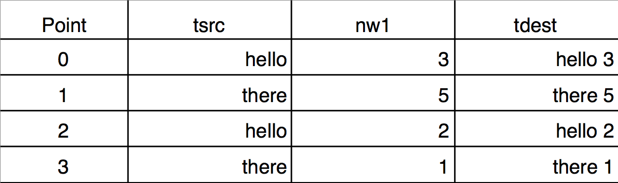
Single-key text sort:

Sort tsrc,tdest	// nw1 not used

Execute this to scramble tdest again:

tdest= tsrc + " " + num2str(nw1)

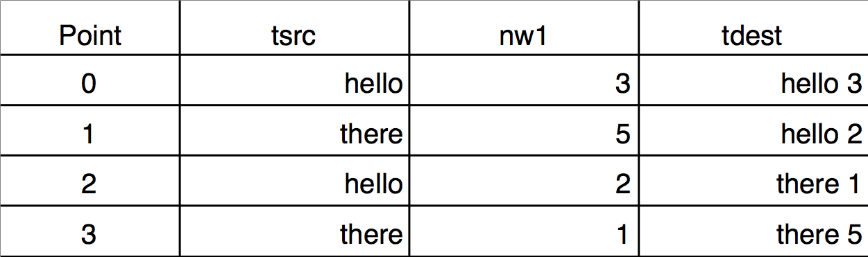
Execute this to see a two key sort (nw1 breaks ties):

Sort {tsrc,nw1},tdest

The reason that "hello 3" sorts after "hello 2" is because nw1[0] = 3 is greater than nw1[2] = 2.

You can sort by more than two keys by specifying more than two waves inside the braces.

MakeIndex and IndexSort

The MakeIndex and IndexSort operations are infrequently used. You will normally use the Sort operation.

Applications of MakeIndex and IndexSort include:

• Sorting large quantities of data

• Sorting individual waves from a group one at a time

• Accessing data in sorted order without actually rearranging the data

• Restoring data to the original ordering

The MakeIndex operation creates a set of index numbers. IndexSort can then use the index numbers to rearrange data into sorted order. Together they can be used to sort just like the Sort operation but with an extra wave and an extra step.

The advantage is that once you have the index wave you can quickly sort data from a given set of waves at any time. For example, if you have hundreds of waves you cannot use the normal sort operation on a single command line. Also, when writing procedures it is sometimes more convenient to loop through a set of waves one at a time than to try to generate a single command line with multiple waves.

You can also use the index values to access data in sorted order without using the IndexSort operation. For example, if you have data and index waves named wave1 and wave1index, you can access the data in sorted order on the right hand side of a wave assignment like so:

wave1[wave1index[p]]

Like the Sort operation, the MakeIndex operation can handle multiple sort keys.

The output wave from MakeIndex contains indices which can be used to access the elements of the input wave in sorted order. These indices can be used later with IndexSort to sort the input wave and/or to reorder other waves. For example:

Make/O data0 = {1,9,2,3}
Make/O/N=4 index
MakeIndex data0, index
Print index		// Prints 0, 2, 3, 1

The output values 0, 2, 3, and 1 mean that, to sort data0, you would access element 0, then element 2, then element 3, then element 1. For example, this prints the values of data0 in order:

Print data0[0], data0[2], data0[3], data0[1]

You can now apply that sequence of access using IndexSort:

IndexSort index, data0
Print data0		// Prints 1, 2, 3, 9

You can apply the same reordering to another wave using IndexSort:

Make/O data1 = {0,1,2,3}
IndexSort index, data1
Print data1		// Prints 0, 2, 3, 1

Decimation

If you have a large data set it may be convenient to deal with a smaller but representative number of points. In particular, if you have a graph with millions of points, it probably takes a long time to draw or print the graph. You can do without many of the data points without altering the graph much. Decimation is one way to accomplish this.

There are at least two ways to decimate data:

1. Keep only every nth data value. For example, keep the first value, discard 9, keep the next, discard 9 more, etc. We call this Decimation by Omission.

2. Replace every nth data value with the result of some calculation such as averaging or filtering. We call this Decimation by Smoothing.

Decimation by Omission

To decimate by omission, create the smaller output wave and use a simple Waveform Arithmetic and Assignment statement to set their values. For example, If you are decimating by a factor of 10 (omitting 9 out of every 10 values), create an output wave with 1/10th as many points as the input wave.

For example, make a 1000 point test input waveform:

Make/O/N=1000 wave0
SetScale x 0, 5, wave0
wave0 = sin(x) + gnoise(.1)

Now, make a 100 point waveform to contain the result of the decimation:

Make/O/N=100 decimated
SetScale x 0, 5, decimated	// preserve the x range
decimated = wave0[p*10]	// for(p=0;p<100;p+=1) decimated[p]= wave0[p*10]

Decimation by omission can be obtained more easily using the Resample operation and dialog by using an interpolation factor of 1 and a decimation factor of (in this case) 10, and a filter length of 1.

Duplicate/O wave0, wave0Resampled
Resample/DOWN=10/N=1 wave0Resampled

Decimation by Smoothing

While decimation by omission completely discards some of the data, decimation by smoothing combines all of the data into the decimated result. The smoothing can take many forms: from simple averaging to various kinds of lowpass digital filtering.

The simplest form of smoothing is averaging (sometimes called "boxcar" smoothing). You can decimate by averaging some number of points in your original data set. If you have 1000 points, you can create a 100 point representation by averaging every set of 10 points down to one point. For example, make a 1000 point test waveform:

Make/O/N=1000 wave0
SetScale x 0, 5, wave0
wave0 = sin(x) + gnoise(.1)

Now, make a 100 point waveform to contain the result of the decimation:

Make/O/N=100 wave1
SetScale x 0, 5, wave1
wave1 = mean(wave0, x, x+9*deltax(wave0))

Notice that the output wave, wave1, has one tenth as many points as the input wave.

The averaging is done by the waveform assignment

wave1 = mean(wave0, x, x+9*deltax(wave0))

This evaluates the right-hand expression 100 times, once for each point in wave1. The symbol "x" returns the X value of wave1 at the point being evaluated. The right-hand expression returns the average value of wave0 over the segment that corresponds to the point in wave1 being evaluated.

It is essential that the X values of the output wave span the same range as the X values of the input range. In this simple example, the SetScale commands satisfy this requirement.

Results similar to the example above can be obtained more easily using the Resample operation and dialog.

Resample is based on a general sample rate conversion algorithm that optionally interpolates, low-pass filters, and then optionally decimates the data by omission. The lowpass filter can be set to "None" which averages an odd number of values centered around the retained data points. So decimation by a factor of 10 would involve averaging 11 values centered around every 10th point.

The decimation by averaging above can be changed to be 11 values centered around the retained data point instead 10 values from the beginning of the retained data point this way:

Make/O/N=100 wave1Centered
SetScale x 0, 5, wave1Centered
wave1Centered = mean(wave0, x-5*deltax(wave0), x+5*deltax(wave0))

Each decimated result (each average) is formed from different values than wave1 used, but it isn't any less valid as a representation of the original data.

Using the Resample operation:

Duplicate/O wave0, wave2
Resample/DOWN=10/WINF=None/N=11 wave2		// no /UP means no interpolation

gives nearly identical results to the wave1Centered = mean(...) computation, the exceptions being only the initial and final values, which are simple end-effect variations.

The /WINF and /N flags of Resample define simple low-pass filtering options for a variety of decimation-by-smoothing choices. The default /WINF=Hanning window gives a smoother result than /WINF=None. See WindowFunction operation for more about these window options.

See Multidimensional Decimation for a discussion of decimating 2D and higher dimension waves.

Miscellaneous Operations

Using WaveTransform

When working with large amounts of data (many waves or multiple large waves), it is frequently useful to replace various wave assignments with wave operations which execute significantly faster. The WaveTransform operation is designed to help in these situations. For example, to flip the data in a 1D wave you can execute the following code:

Function FlipWave(inWave)
	wave inWave
	
	Variable num=numPnts(inWave)
	Variable n2=num/2
	Variable i,tmp
	num-=1
	Variable j
	for(i=0;i<n2;i+=1)
		tmp=inWave[i]
		j=num-i
		inWave[i]=inWave[j]
		inWave[j]=tmp
	endfor
End

You can obtain the same result much faster using the command:

WaveTransform/O flip, waveName

In addition to "flip", WaveTransform can also fill a wave with point index or the inverse point index, shift data points, normalize, convert to complex-conjugate, compute the squared magnitude or the phase, etc.

For multi-dimensional waves, use MatrixOp instead of WaveTransform. See Using MatrixOp for details.

The Compose Expression Dialog

The Compose Expression item in the Analysis menu brings up the Compose Expression dialog.

This dialog generates a command which sets the value of a wave, variable or string based on a numeric or string expression created by pointing and clicking. Any command that you can generate using the dialog could also be typed directly into the command line.

The command that you generate with the Compose Expression dialog consists of three parts: the destination, the assignment operator and the expression. The command resembles an equation and is of the form:

<destination> <assignment-operator> <expression>

For example:

wave1 = K0 + wave2         // a wave assignment command
K0 += 1.5 * K1             // a variable assigment command
str1 = "Today is" + date() // a string assignment command

Table Selection Item

The Destination Wave pop-up menu contains a "_table selection_" item. When you choose "_table selection_", Igor assigns the expression to whatever is selected in the table. This could be an entire wave or several entire waves, or it could be a subset of one or more waves.

To use this feature, start by selecting in a table the numeric wave or waves to which you want to assign a value. Next, choose Compose Expression from the Analysis menu. Choose "_table selection_" in the Destination Wave pop-up menu. Next, enter the expression that you want to assign to the waves. Notice the command that Igor has created which is displayed in the command box toward the bottom of the dialog. If you have selected a subset of a wave, Igor will generate a command for that part of the wave only. Finally, click Do It to execute the command.

Create Formula Checkbox

The Create Formula checkbox in the Compose Expression dialog makes Igor generate a command using the := operator rather than the = operator. The := operator establishes a dependency such that, if a wave or variable on the right hand side of the assignment statement changes, Igor will reassign values to the destination (left hand side). We call the right hand side a formula. Dependencies provides details on dependencies and formulas.

Matrix Math Operations

There are four basic methods for performing matrix calculations: normal wave expressions, the MatrixXXX operations, the MatrixOp operation, and the MatrixSparse operation.

Normal Wave Expressions

You can add matrices to other matrices and scalars using normal wave expressions. You can also multiply matrices by scalars. For example:

Make matA={{1,2,3},{4,5,6}}, matB={{7,8,9},{10,11,12}}
matA = matA+0.01*matB

gives new values for

matA = {{1.07,2.08,3.09},{4.1,5.11,6.12}}

MatrixXXX Operations

A number of matrix operations are implemented in Igor. Most have names starting with the word "Matrix". For example, you can multiply a series of matrices using the MatrixMultiply operation. The /T flag allows you to specify that a given matrix's data should be transposed before being used in the multiplication.

Many of Igor's matrix operations use the LAPACK library. To learn more about LAPACK see:

LAPACK Users' Guide, Third Edition, 1999 (SIAM Publications, Philadelphia, ISBN: 0-89871-447-8)

or the LAPACK web site:

http://www.netlib.org/lapack/lug/lapack_lug.html

Unless noted otherwise, LAPACK routines support real and complex, IEEE single-precision and double-precision matrix waves. Most matrix operations create the variable V_Flag and set it to zero if the operation is successful. If the flag is set to a negative number it indicates that one of the parameters passed to the LAPACK routines is invalid. If the flag value is positive it usually indicates that one of the rows/columns of the input matrix caused the problem.

MatrixOp Operation

The MatrixOp operation improves the execution efficiency and simplifies the syntax of matrix expressions. For example, the command

MatrixOp matA = (matD - matB x matC) x matD

is equivalent to matrix multiplications and subtraction following standard precedence rules.

See Using MatrixOp for details.

MatrixSparse Operation

The MatrixSparse operation can improve performance and reduce memory utilization for calculations involving large matrices the elements of which are mostly 0. See Sparse Matrices for details.

Matrix Commands

Here are the matrix math operations and functions:

General

• MatrixCondition(matrix )
• MatrixConvolve coefMatrix, dataMatrix
• MatrixCorr [/COV][/DEGC] waveA [, waveB ]
• MatrixDet(matrix )
• MatrixDot(waveA, waveB )
• MatrixFilter [/N=n /P=p /b=b /R=roiWave ] Method dataMatrix
• MatrixGLM [/Z] matrixA, matrixB, waveD
• MatrixMultiply matrixA [/T],matrixB [/T] [,additional matrices]
• MatrixOp [/O] destwave = expression
• MatrixRank(matrix [, maxConditionNumber ])
• MatrixTrace(matrix )
• MatrixTranspose matrix

EigenValues, Eigenvectors and Decompositions

• MatrixBalance [flags] srcWave
• MatrixEigenV [/O/B=balance /S=sense /X/R/L/Z] matrixWave
• MatrixFactor [flags] srcWave
• MatrixGLM matrixA, matrixB, waveD
• MatrixInverse [[/D]/P][/G][/O] srcWave
• MatrixLUD matrix
• MatrixLUDTD srcMain, srcUpper, srcLower
• MatrixReverseBalance [flags] scaleWave, eigenvectorsWave
• MatrixSchur [/Z] matrix
• MatrixSVD matrix

Linear Equations and Least Squares

• MatrixGaussJ matrixA, vectorsB
• MatrixLinearSolve [/D={subDiagonals,superDiagonals }/M=method /O/Z] [/L][/U] matrixA, matrixB
• MatrixLinearSolveTD [/Z] upperW, mainW, lowerW, matrixB
• MatrixLLS [/O/Z/M=method ] matrixA, matrixB
• MatrixLUBkSub matrtixL, matrixU, index, vectorB
• MatrixSolve method, matrixA, vectorB
• MatrixSVBkSub matrixU, vectorW, matrixV, vectorB

Sparse Matrices

• MatrixSparse

Using MatrixOp

When performing mathematical calculations your first choice may be to write standard wave assignments such as:

wave1 = wave2 + wave3

When the expression on the right-hand-side (RHS) is complicated or when the waves are large you can gain a significant performance improvement using MatrixOp (short for "matrix operation"). MatrixOp was originally conceived to perform calculations on 2D waves and was later extended to waves of any dimension.

To use the basic form of MatrixOp simply prepend its name to the assignment statement:

MatrixOp wave1 = wave2 + wave3

Although the two commands appear similar, having the general form:

destWave = expression

they are different in behavior.

A significant difference is that MatrixOp operates on pure array elements without regard to wave scaling and does not support indexing using x, y, z, t, p, q, r, or s on the RHS.

The wave assignment requires that the destination wave exist at the time of execution but MatrixOp creates its destination wave automatically. In these commands:

Make/O wave2 = 1/(p+1), wave3 = 1
MatrixOp/O wave1 = wave2 + wave3

MatrixOp creates a single precision (SP) wave named wave1 and stores the result in it.

When MatrixOp creates a destination wave, its data type and dimensions depend on the expression on the RHS. In the preceding example, MatrixOp created wave1 as SP because wave2 and wave3 are SP. The rules that MatrixOp uses to determine the data type and dimensions of the destination are discussed below under MatrixOp Data Promotion Policy.

These rules leads to the following difference between MatrixOp and wave assignments:

Make/O wave1 = 42		// wave1 is 128 points wave, all points are set to 42
MatrixOp/O wave1 = 42	// wave1 is now 1 point wave set to 42

Assignment statements evaluate the RHS and store the result in a point-by-point manner. Because of this, you sometimes get unexpected results if the destination wave appears on the RHS. In this example, WaveMin(wave2) changes during the evaluation of the assignment statement:

wave2 = wave2 - WaveMin(wave2)

By contrast, MatrixOp evaluates the RHS for all points in the destination before storing anything in the destination wave. Consequently this command behaves as expected:

MatrixOp/O wave2 = wave2 - minVal(wave2)

Another important difference appears when the RHS involves complex numbers. If you try, for example,

Make/O/C cwave2
Make/O wave1, wave3
wave1 = cwave2 + wave3

you get an error, "Complex wave used in real expression".

By contrast, MatrixOp creates the destination as complex so this command works without error:

MatrixOp/O wave1 = cwave2 + wave3

In this example the RHS mixes real and complex waves, something MatrixOp handles without problems.

In addition to the standard math operators, MatrixOp supports a list of functions that can be applied to operands on the RHS. Examples are abs, sin, cos, mean, minVal and maxVal. There are many more described in the MatrixOp reference documentation and listed below under MatrixOp Functions by Category.

MatrixOp Data Tokens

A MatrixOp command has the general form:

MatrixOp [flags] destWave = expression

The expression on the RHS is a combination of data tokens with MatrixOp operators and MatrixOp functions. A data token is one of the following:

• A literal number

• A numeric constant declared with the Constant keyword

• A numeric local variable

• A numeric global variable

• A numeric wave

• A numeric wave layer

• The result from a MatrixOp function

You cannot call a user-defined function or external function from expression.

This function illustrates each type of data token:

Constant kConstant = 234
Function Demo()
	// Literal number
	MatrixOp/O dest = 123
	
	// Constant
	MatrixOp/O dest = kConstant
	
	// Local Variable
	Variable localVariable = 345
	MatrixOp/O dest = localVariable
	
	// Global Variable
	Variable/G root:gVar = 456
	NVAR globalVariable = root:gVar
	MatrixOp/O dest = globalVariable
	
	// Wave
	Make/O/N=(3,3) mat = p + 10*q
	MatrixOp/O tMat = mat^t
	
	// Wave layer
	Make/O/N=(3,3,3) w3D = p + 10*q + 100*r
	MatrixOp/O layer1 = w3D[][][1]

	// Output from a MatrixOp function
	MatrixOp/O invMat = inv(mat)
End

MatrixOp Wave Data Tokens

MatrixOp uses only the numeric data and the dimensions of waves. All other properties, in particular wave scaling, are ignored. If wave scaling is important in your application, follow MatrixOp with CopyScales or SetScale or use a wave assignment statement instead of MatrixOp.

From the command line you can reference a wave in expression using the simple wave name, the partial data folder path to the wave or the full data folder path to a wave. In a user-defined function you can reference a wave using a simple wave or a wave reference variable pointing to an existing wave. We call all of these methods of referencing waves "wave references".

A wave data token consists of a wave reference optionally qualified by indices that identify a subset of the wave. For example:

Function Demo()
	// Creates automatic wave reference for w3D
	Make/O/N=(3,4,5) w3D = p + 10*q + 100*r

	MatrixOp/O dest = w3D            // dest is a 3D wave
	MatrixOp/O dest = w3D[0][1][2]   // dest is a 1D wave with 1 point
	MatrixOp/O dest = w3D[0][1][]    // dest is a 2D wave with 1 layer
End

MatrixOp supports only two kinds of subsets of waves:

• A subset that evaluates to a scalar (a single value)

• A subset that evaluates to one or more layers (2D arrays)

Subsets that evaluate to a row (w3D[1][][2]) or a column (w3D[][1][2]) are not supported.

Scalars: The following expressions evaluate to scalars:

wave1d[a]	a is a literal number or a local variable. MatrixOp clips the index a to the valid range for wave1d. The expression evaluates to a scalar equal to the referenced wave element.
wave2d[a][b]	a and b are literal numbers or local variables. MatrixOp clips the indices to the valid range of the corresponding dimensions. The expression evaluates to a scalar equal to the referenced wave element.
wave3d[a][b][c]	a, b and c are literal numbers or local variables. MatrixOp clips the indices to the valid range of the corresponding dimensions. The expression evaluates to a scalar equal to the referenced wave element.

Layers: The following evaluate to one or more 2D layers:

wave3d[][][a]	Layer a from the 3D wave is treated as a 2D matrix. The first and second bracket pairs must be empty. MatrixOp clips a to the valid range of layers. The result is a 2D wave.
wave3d[][][a,b]	expression is evaluated for all layers between layer a and layer b. MatrixOp clips a and b to the valid range of layers. The result is a 3D wave.
wave3d[][][a,b,c]	expression is evaluated for layers starting with layer a and increasing to layer b incrementing by c. a, b and c must be scalars. Layers are clipped to the valid range and c must be a positive integer.

You can use waves of any dimensions as parameters to MatrixOp functions. For example:

Make/O/N=128 wave1d = x
MatrixOp/O outWave = exp(wave1d)

MatrixOp does not support expressions that include the same 3D wave on both sides of the equation:

MatrixOp/O wave3D = wave3D + 3	// Not allowed
Instead use:
MatrixOp/O newWave3D = wave3D + 3

You can use any combination of data types for operands. In particular, you can mix real and complex types in expression. MatrixOp determines data types of inputs and the appropriate output data type at runtime without regard to any type declaration such as Wave/C.

MatrixOp functions can create certain types of 2D data tokens. The const and zeroMat functions create matrices of specified dimensions containing fixed values. The identity function creates identity matrixes and triDiag creates a tridiagonal matrix from 1D input waves. The rowRepeat and colRepeat functions also construct matrices from 1D waves. The setRow, setCol and setOffDiag functions transfer data from 1D waves to elements of 2D waves.

MatrixOp and Wave Dimensions

MatrixOp was designed to optimize operations on 2D arrays (matrices) but it also supports other wave dimensions in various expressions. However it does not support zero point waves.

A 1D wave is treated as a matrix with one column. 3D and 4D waves are treated as arrays of layers so their assignments are processed on a layer-by-layer basis. For example:

Make/O/N=(4,5) wave2 = q
Make/O/N=(4,5,6) wave3 = r
MatrixOp/O wave1 = wave2 * wave3	// 2D multiplies 3D one layer at a time

wave1 winds up as a 3D wave of dimensions (4,5,6). Each layer in wave1 contains the contents of the corresponding layer in wave3 multiplied on an element-by-element basis by the contents of wave2.

Exceptions for layer-by-layer processing are special MatrixOp functions such as beam and transposeVol.

Some binary operators have dimensional restrictions for their wave operands. For example, matrix multiplication (wave2 x wave3) requires that the number of columns in wave2 be equal to the number of rows in wave3. Regular multiplication (wave2*wave3) requires that the number of rows and the columns of the two be equal. For example,

Make/O/N=(4,6) wave2
Make/O/N=(3,8) wave3
MatrixOp/O wave1 = wave2 * wave3		// Error: "Matrix Dimensions Mismatch"

The exception to this rule is when the righthand operand is a single wave element:

MatrixOp/O wave1 = wave2 * wave3[2][3]	// Equivalent to scalar multiplication

Some MatrixOp functions operate on each column of the matrix and result in a 1 row by N column wave which may be confusing when used elsewhere in Igor. If what you need is an N row 1D wave you can redimension the wave or simply include a transpose operator in the MatrixOp command:

Make/O/N=(4,6) wave2=gnoise(4)
MatrixOp/O wave1=sumCols(wave2)^t	// wave1 is a 1D wave with 6 rows

MatrixOp Operators

MatrixOp defines 8 binary operators and two postfix operators which are available for use in the RHS expression. The operators are listed in the Operators section of the reference documentation for MatrixOp.

MatrixOp does not support operator combinations such as +=.

The basic operators, +, -, *, and /, operate in much the same way as they would in a regular wave assignment with one exception: when the - or / operation involves a matrix and a scalar, it is only supported if the matrix is the first operand and the scalar is the second. For example:

Make/O wave2 = 1
Variable var1 = 7
MatrixOp/O wave1 = wave2 - var1	// OK: Subtract var1 to each point in wave2
MatrixOp/O wave1 = var1 - wave2	// Error: Can't subtract a matrix from a scalar
MatrixOp/O wave1 = var1 / wave2	// Error: Can't divide a scalar by a matrix

Division of a scalar by a matrix can be accomplished using the reciprocal function as in:

MatrixOp/O wave1 = scalar * rec(wave2)

The dot operator . is used to compute the generalized dot product:

MatrixOp/O wave1 = wave2 . wave3	// Spaces around '.' are optional

The x operator designates matrix-matrix multiplication.

MatrixOp/O wave1 = wave2 x wave3	// Spaces around 'x' are required!

The logical operators && and || are restricted to real-valued data tokens and produce unsigned byte numeric tokens with the value 0 or 1.

The two postfix operators ^t (matrix transpose) and ^h (Hermitian transpose) operate on the first token to their left:

MatrixOp/O wave1 = wave2^t + wave3

The transpose operation has higher precedence and thus is executed before the addition.

The left token may be a compound token as in:

MatrixOp/O wave1 = sumCols(wave2)^t

MatrixOp supports the ^ character only in the two postfix operators ^t and ^h. For exponentiation use the powR and powC functions.

MatrixOp Multiplication and Scaling

MatrixOp provides a number of multiplication and scaling capabilities. They include matrix-scalar multiplication:

MatrixOp/O wave1 = wave2 * scalar	// Equivalent to a wave assignment

and wave-wave multiplication:

MatrixOp wave1 = wave2 * wave3	// Also includes layer-by-layer support

and matrix-matrix multiplication:

MatrixOp wave1 = wave2 x wave3

The latter is equivalent to the MatrixMultiply operation with the convenience of allowing you to write and execute complicated compound expressions in one line.

MatrixOp adds two specialized scaling functions that are frequently used. The scaleCols function multiplies each column by a different scalar and the scale function scales its input to a specified range.

MatrixOp Data Rearrangement and Extraction

MatrixOp is often used to rearrange data in a matrix or to extract a subset of the data for further calculation. You can extract an element or a layer from a wave using square-bracket indexing:

MatrixOp destWave = wave1d[a]       // Extract scalar from point a of the wave
MatrixOp destWave = wave2d[a][b]    // Extract scalar from element a,b of the wave
MatrixOp destWave = wave3d[a][b][c] // Extract scalar from element a,b,c of the wave
MatrixOp destWave = wave3d[][][a]   // Extract layer a from the 3D wave

You can also extract layers from a 3D wave starting with layer a and increasing the layer number up to layer b using increments c:

MatrixOp destWave = wave3d[][][a,b,c]

a, b and c must be scalars. Layers are clipped to the valid range and c must be a positive integer.

If you need to loop over rows, columns, layers or chunks it is often useful to extract the relevant data using the MatrixOp functions row, col, layer and chunk. You can extract matrix diagonals using getDiag. You can use subRange to extract more than one row or more than one column.

The Rotate operation works on 1D waves. MatrixOp extends this to higher dimensions with the functions: rotateRows, rotateCols, rotateLayers, and rotateChunks.

MatrixOp transposeVol is similar to ImageTransform transposeVol but it supports complex data types.

The MatrixOp redimension function is designed to convert 1D waves into 2D arrays but it can also extract data from higher-dimensional waves.

MatrixOp Data Promotion Policy

MatrixOp chooses the data type of the destination wave based on the data types and operations used in the expression on the RHS. Here are some examples:

Make/O/B/U wave2, wave3          // Create two unsigned byte waves
MatrixOp/O wave1 = wave2         // wave1 is unsigned byte
MatrixOp/O wave1 = wave2 + wave3 // wave1 is unsigned word (16 bit)
MatrixOp/O wave1 = wave2 * wave3 // wave1 is unsigned word (16 bit)
MatrixOp/O wave1 = wave2 / wave3 // wave1 is SP
MatrixOp/O wave1 = magsqr(wave2) // wave1 is SP

The examples show the destination wave's data type changing to represent the range of possible results of the operation. MatrixOp does not inspect the data in the waves to determine if the promotion is required for the specific waves.

Igor variables are usually treated as double precision data tokens. MatrixOp applies special rules for variables that contain integers. Here is an example:

Make/O/B/U wave2              // Create unsigned byte wave
Variable vv = 2.1             // Variable containing DP value
MatrixOp/O wave1 = wave2*vv   // wave1 is DP

Now change the variable to store various integers:

vv = 2
MatrixOp/O wave1 = wave2*vv   // wave1 is unsigned word (16 bit)
vv = 257
MatrixOp/O wave1 = wave2*vv   // wave1 is unsigned integer (32 bit)
vv = 65538
MatrixOp/O wave1 = wave2*vv   // wave1 is DP

These examples show that MatrixOp represents the variable vv as a token with a data type that fits it contents. If the variable does not contain an integer value the token is treated as DP.

MatrixOp is convenient for complex math calculations because it automatically creates real or complex destination waves as appropriate. For example:

Make/O/C wave2, wave3                        // SP complex
Make/O wave4                                 // SP real
MatrixOp/O wave1 = wave2 * wave3 * wave4     // wave1 is SP complex
MatrixOp/O wave1 = abs(wave2*wave3) * wave4  // wave1 is SP real

An exception to the complex policy is the sqrt function which returns NaN when its input is real and negative.

If you want to restrict data type promotion you can use the /NPRM flag:

Make/O/B/U wave2, wave3
MatrixOp/O wave1 = wave2 * wave3       // wave1 is unsigned word (16 bit).
MatrixOp/O/NPRM wave1 = wave2 * wave3  // wave1 is unsigned byte

A number of MatrixOp functions convert integer tokens to SP prior to processing and are not affected by the /NPRM flag. These include all the trigonometric functions, chirp and chirpZ, fft, ifft, normalization functions, sqrt, log, exp and forward/backward substitutions.

MatrixOp Compound Expressions

You can use compound expressions with most MatrixOp functions that operate on regular data tokens. In a compound expression you pass the result from one MatrixOp operator or function as the input to another. For example:

MatrixOp/O wave1 = sum(abs(wave2-wave3))

This is particularly convenient for transformations and filtering:

MatrixOp/O wave1 = IFFT(FFT(wave1,2)*filterWave,3)

Some MatrixOp functions, such as beam and transposeVol, do not support compound expressions because they require input that has more than two-dimensions while compound expressions are evaluated on a layer by layer basis:

Make/O/N=(10,20,30) wave3
MatrixOp/O wave1 = beam(wave3+wave3,5,5)  // Error: Bad MatrixOp token
MatrixOp/O wave1 = beam(wave3,5+1,5)      // Compound expression allowed here

MatrixOp Quaternion Data Tokens

A quaternion {w,x,y,z} consists of an amplitude w and three vector components x, y, and z where:

w = a, x = bi, y = cj, z = dk

a, b, c and d are real numbers. i, j, and k are the fundamental quaternion units, analogous to i in complex numbers.

Quaternions are often used to represent rotation in 3D graphics. Igor Pro 8 added support for quaternions via MatrixOp functions.

Quaternion arithmetic has its own rules. For example, multiplication is not commutative (ij is not equal to ji).

You can do quaternion arithmetic with MatrixOp by creating and then manipulating quaternion tokens. For example:

Function QuaternionMultiplicationDemo()
	// Create waves containing the w, x, y, and z values of quaternions
	Make/FREE wR = {1, 0, 0, 0}
	Make/FREE wI = {0, 1, 0, 0}
	Make/FREE wJ = {0, 0, 1, 0}
	Make/FREE wK = {0, 0, 0, 1}
	
	MatrixOp/O rW = quat(wR) * quat(wI)	// rW is the result wave
	Printf "1i = {%g,%g,%g,%g} (i)\r", rW[0], rW[1], rW[2], rW[3]
	
	MatrixOp/O rW = quat(wI) * quat(wI)
	Printf "ii = {%g,%g,%g,%g} (-1)\r", rW[0], rW[1], rW[2], rW[3]
	
	MatrixOp/O rW = quat(wI) * quat(wJ)
	Printf "ij = {%g,%g,%g,%g} (k)\r", rW[0], rW[1], rW[2], rW[3]
	
	MatrixOp/O rW = quat(wJ) * quat(wI)
	Printf "ji = {%g,%g,%g,%g} (-k)\r", rW[0], rW[1], rW[2], rW[3]
End

In this example, wR, wI, wJ and wK are waves containing the w, x, y, and z values of quaternions. rW is the result wave from MatrixOp. quat(wR), quat(wI) and quat(wJ) are MatrixOp quaternion tokens. They exist only during the execution of a MatrixOp command. MatrixOp uses quaternion arithmetic to evaluate expressions containing quaternion tokens. After the righthand side has been evaluated, MatrixOp stores the result in a wave. Functions that return quaternion coordinates, such as quat and matrixToQuat, return a 4-element wave containing the w, x, y and z values.

You can also create a quaternion token from a scalar or from a wave containing x, y, and z values:

Function QuaternionTokenDemo()
	Make/FREE wI = {0, 1, 0, 0}   // w, x, y, z
	Make/FREE wXYZ = {1, 0, 0}    // x, y, z
	
	MatrixOp/O rW = quat(wI) * quat(wXYZ)
	Printf "ii = {%g,%g,%g,%g} (-1)\r", rW[0], rW[1], rW[2], rW[3]

	MatrixOp/O rW = quat(wI) * quat(wXYZ) * quat(3)
	Printf "3ii = {%g,%g,%g,%g} (-3)\r", rW[0], rW[1], rW[2], rW[3]
End

quat(wXYZ) converts the wave containing x, y, and z to a pure imaginary quaternion whose w component is 0. wXZY can be a 3x1 wave as in this example or it can be a 1x3 wave; both produce the same quaternion token.

quat(3) converts the scalar value 3 to a real quaternion whose x, y and z components are 0.

The input to quat must be real, not complex.

The quat function does not normalize the quaternion. It is normalized when it is used as an input to another MatrixOp quaternion operation.

MatrixOp supports the following quaternion functions:

quat, quatToMatrix, quatToAxis, axisToQuat, quatToEuler, and slerp

These are documented in the reference documenation for MatrixOp.

This example shows how to use quatToEuler to generale Euler angles from a quaternion:

Function QuaternionEulerDemo()
	Make/FREE wI = {0, 1, 0, 0}
	MatrixOp/O rW = quatToEuler(quat(wI), 123)
	Printf "Euler angles = {%g,%g,%g}\r", rW[0], rW[1], rW[2]
End

MatrixOp Multithreading

Common CPUs are capable of running multiple threads. Some calculations are well suited to run in parallel. There are a several ways to take advantage of multithreading using MatrixOp:

• User-created preemptive threads

  MatrixOp is thread-safe so you can call it from preemptive threads. See ThreadSafe Functions and Multitasking for details.

• Layer threads

  If you are evaluating expressions that involve multiple layers you can use the /NTHR flag to run each layer calculation in a separate thread. When you account for thread overhead it makes sense to use /NTHR when the per-layer calculations are on the order of 1 million CPU cycles or more.

• Internal multithreading of operations or functions

  Some MatrixOp functions are automatically multithreaded for SP and DP data. These include matrix-matrix multiplication, trigonometric functions, hypot, sqrt, erf, erfc, inverseErf, and inverseErfc. The MultiThreadingControl operation provides fine-tuning of automatic multithreading but you normally do not need to tinker with it.

MatrixOp Performance

In most situations MatrixOp is faster than a wave assignment or FastOp. However, for small waves, the extra overhead may make it slower.

MatrixOp works fastest on floating point data types. For maximum speed, convert integer waves to single-precision floating point before calling MatrixOp.

Some MatrixOp expressions are evaluated with automatic multithreading. See MatrixOp Multithreading for details.

MatrixOp Optimization Examples

The section shows examples of using MatrixOp to improve performance.

• Replace matrix manipulation code with MatrixOp calls. For example, replace this:

  		Make/O/N=(vecSize,vecSize) identityMatrix = p==q ? 1 : 0
  		MatrixMultiply matB, matC
  		identityMatrix -= M_Product
  		MatrixMultiply identityMatrix, matD
  		MatrixInverse M_Product
  		Rename M_Inverse, matA

  with:

  		MatrixOp matA = Inv((Identity(vecSize) - matB x matC) x matD)

• Replace waveform assignment statements with MatrixOp calls. For example, replace this:

  		Duplicate/O wave2,wave1
  		wave1 = wave2*2

  with:

  		MatrixOp/O wave1 = wave2*2

• Factor and compute only once any repeated sub-expressions. For example, replace this:

  		MatrixOp/O wave1 = var1*wave2*wave3
  		MatrixOp/O wave4 = var2*wave2*wave3

  with:

  		MatrixOp/O/FREE tmp = wave2*wave3	// Compute the product only once
  		MatrixOp/O wave1 = var1*tmp
  		MatrixOp/O wave4 = var2*tmp

• Replace instances of the ?: conditional operator in wave assignments with MatrixOp calls. For example, replace this:

  		wave1 = wave1[p]==0 ? NaN : wave1[p]

  with:

  		MatrixOp/O wave1 = setNaNs(wave1,equal(wave1,0))

MatrixOp Functions by Category

This section lists the MatrixOp functions by category to help you select the appropriate function.

Numbers and Arithmetic

e	enoise	inf	Pi	nan	maxAB
minAB	maxMagAB	minMagAB	mod

Trigonometric

acos	asin	atan	atan2	cos	hypot
phase	sin	sqrt	tan

Exponential

acosh	asinh	atanh	cosh	exp	expIntegralE1
expm	ln	log	powC	powR
sinh	tanh

Complex

cmplx	conj	imag	magSqr	p2Rect	phase
powC	r2Polar	real

Rounding and Truncation

abs	ceil	clip	floor	limit	mag
round

Conversion

cmplx
fp32	fp64
int8	int16	int32	uint8	uint16	uint32

Data Properties

numCols	numPoints	numRows	numType
waveChunks	waveLayers	wavePoints
waveX	waveY	waveZ	waveT

Data Characterization

averageCols	binMean	binVar	crossCovar	chol	det
frobenius	integrate	indexCols	indexRows	intMatrix
maxCols	maxRows	maxVal
mean	minCols	minRows	minVal
normP	oneNorm
productCol	productCols	productDiagonal	productRows
sgn
sum	sumBeams	sumCols	sumND	sumRows	sumSqr
trace	varBeams	varCols

Data Creation and Extraction

beam	catCols	catRows	col	colRepeat	rowRepeat
chunk	const	decimateMinMax	getDiag	identity	insertMat
IndexMatch	inv	layer	layerStack	rec	removeCol
removeCols	setType	subRange	subWaveC	subWaveR
tridiag	waveIndexSet	waveMap	zeroMat

Data Transformation

addCols	addRows	bitReverseCol	diagonal	diagRC
median	normalize	normalizeCols	normalizeRows
redimension	replace	replaceNaNs	replaceInfs
reverseCol	reverseCols	reverseRow	reverseRows
rotateChunks	rotateCols	rotateLayers	rotateRows	rowDiff
scale	scaleCols	spliceCols	scaleChunks	scaleLayers
setCol	setColsRange	setNaNs	setOffDiag	setRow
shiftVector	subtractCols	subtractMean	subtractMin	subtractRows
transposeVol	zapINFs	zapNaNs	zapZeros

Time Domain

asyncCorrelation	convolve	correlate	limitProduct	syncCorrelation

Frequency Domain

chirpZ	chirpZf	fft	ifft
FST	FCT	FSST	FSCT
FSST2	FSCT2

Matrix

backwardSub	chol	covariance	det	diagonal
diagRC	forwardSub	frobenius	getDiag	identity
inv	kronProd	outerProduct	setOffDiag	tensorProduct
trace

Special Functions

erf	erfc	gamma	gammaln	inverseErf	inverseErfc

Logical

equal	greater	within

Bitwise

bitAnd	bitOr	bitShift	bitXOR	bitNot

Quaternions

quat	axisToQuat	quatToAxis	matrixToQuat	quatInverse
quatFromSpherical	quatToMatrix	slerp

Sparse Matrices

Some applications require manipulation of large matrices the elements of which are mostly 0. In these applications, the use of sparse matrices can improve performance and reduce memory utilization.

Igor supports sparse matrices through the MatrixSparse operation which was added in Igor Pro 9.00. It uses the Intel Math Kernel Library Sparse BLAS routines and employs the libraries terminology and conventions.

Sparse Matrix Concepts

In this section we discuss some basic sparse matrix concepts as they apply to Igor. For a general primer on sparse matrices, see https://en.wikipedia.org/wiki/Sparse_matrix.

A normal matrix in Igor is a 2D wave in which each element of the matrix is stored in memory in a regular pattern of rows and columns. In the context of sparse matrices, we use the term "dense matrix" to refer to a normal matrix.

A sparse matrix in Igor is represented by a set of three 1D waves which define the non-zero elements of the matrix. Igor supports three formats, described below, for sparse matrix representation. The formats are called COO (coordinate format), CSC (compressed column format), and CSR (compressed row format). In the following sections, we use the term "sparse matrix" to mean a matrix defined by three 1D waves according to one of these formats.

You can create a sparse matrix equivalent to a dense matrix using the MatrixSparse TOCOO, TOCSR, and TOCSC conversion operations. Alternatively you can create it directly by creating three 1D waves and storing the appropriate values in them. You can create a dense matrix equivalent to a sparse matrix using TODENSE conversion operation.

MatrixSparse supports a number of math operations such as ADD (add two sparse matrices), MV (multiply a sparse matrix by a vector), SMSM (multiply two sparse matrices), and TRSV (solve a system of linear equations).

Sparse matrix operations work on single-precision and double-precision real and complex data. They do not support INFs or NaNs.

Sparse Matrix Formats

A sparse matrix in Igor is represented by a set of three 1D waves which define the non-zero elements of the matrix. Igor supports three sparse matrix storage formats named COO (coordinate format), CSR (compressed row format), and CSC (compressed column format).

MatrixSparse uses the CSR format except for operations that convert between formats.

For the purpose of illustrating these formats, we will use the example dense matrix from the Wikipedia sparse matrix web page:

	0	0	0	0
	5	8	0	0
	0	0	3	0
	0	6	0	0

The term nnz is short for "number of non-zero values" and appears below and in the documentation for MatrixSparse. In this example, nnz = 4.

COO Sparse Matrix Storage Format

"COO" is the shorthand name for "coordinate format". It is conceptually the simplest format and stores each non-zero matrix value along with the corresponding zero-based row and column indices.

In Igor terminology, COO format uses the following three waves:

W_COOValues stores each non-zero value in the matrix.

W_COORows stores the zero-based row index for each non-zero value in the matrix.

W_COOColumns stores the zero-based column index for each non-zero value in the matrix.

Our example matrix is represented in COO format like this:

W_COOValues:   5  8  3  6
W_COORows:     1  1  2  3
W_COOColumns:  0  1  2  1

These values can be read vertically as a set of ordered triplets: (5,1,0), (8,1,1), (3,2,2), and (6,3,1). The last of these tells us that the value 6 is the value of row 3, column 1.

The wave names W_COOValues, W_COORows, and W_COOColumns are used by MatrixSparse when it creates an output sparse matrix in COO format. When you specify an input sparse matrix, you can use any wave names.

CSR Sparse Matrix Storage Format

"CSR" is the shorthand name for "compressed sparse row". It is widely used because it is more efficient in terms of memory use and computational speed than COO.

MatrixSparse uses the CSR format except for operations that convert between formats.

In CSR format, the three 1D waves store the non-zero values, the zero-based column indices, and a "pointer" vector which is used to determine in which row each value appears.

In Igor terminology, CSR format uses the following three waves:

W_CSRValues stores each non-zero value in the matrix.

W_CSRColumns stores the zero-based column index for each non-zero value in the matrix.

W_CSRPointerB stores indices into W_CSRValues which are used to determine in which row a particular value appears.

Our example matrix is represented in CSR format like this:

W_CSRValues:      5  8  3  6
W_CSRColumns:     0  1  2  1
W_CSRPointerB:    0  2  3  4

Unlike the case of COO format, these values cannot be read vertically as a set of ordered triplets. CSR is a bit more complicated.

The first two of these waves can be read as ordered pairs: (5,0), (8,1), (3,2), and (6,1). Each ordered pair specifies a value (e.g., 6) and a column (e.g., 1) but does not tell us in which row the value appears.

The third wave, W_CSRPointerB, is used to determine in which row a given value appears. It contains one index for each row in the represented matrix plus an additional index which is nnz, the number of non-zero values in the matrix. W_CSRPointerB[i] is the zero-based index in W_CSRValues of the first non-zero value in row i.

In this example, we can interpret the values of W_CSRPointerB as follows:

W_CSRPointerB[0] = 0	// The first value for row 0 is at index 0 in W_CSRValues *
W_CSRPointerB[1] = 0	// The first value for row 1 is at index 0 in W_CSRValues
W_CSRPointerB[2] = 2	// The first value for row 2 is at index 2 in W_CSRValues
W_CSRPointerB[3] = 3	// The first value for row 3 is at index 3 in W_CSRValues
W_CSRPointerB[4] = 4	// The number of non-zero values in W_CSRValues is 4

* There are no non-zero values in row 0 so W_CSRPointerB[0] is the same as W_CSRPointerB[1].

When you specify a sparse matrix in CSR format to the MatrixSparse operation, the last element of W_CSRPointerB, specifying nnz, is optional and you can omit it.

The wave names W_CSRValues, W_CSRColumns, and W_CSRPointerB are used by MatrixSparse when it creates an output sparse matrix in CSR format. When you specify an input sparse matrix, you can use any wave names.

CSC Sparse Matrix Storage Format

"CSC" is the shorthand name for "compressed sparse column". It is more efficient in terms of memory use and computational speed than COO.

In CSC format, the three 1D waves store the non-zero values, the zero-based row indices, and a "pointer" vector which is used to determine in which column each value is to be stored.

In Igor terminology, CSC format uses the following three waves:

W_CSCValues stores each non-zero value in the matrix.

W_CSCRows stores the zero-based row indices for each non-zero value in the matrix.

W_CSCPointerB stores indices into W_CSCValues which are used to determine in which column a particular value appears.

The W_CSCPointerB wave works in CSC in a manner analogous to how W_CSRPointerB in CSR.

When you specify a sparse matrix in CSC format to the MatrixSparse operation, the last element of W_CSCPointerB, specifying nnz, is optional and you can omit it.

The wave names W_CSCValues, W_CSCRows, and W_CSCPointerB are used by MatrixSparse when it creates an output sparse matrix in CSC format. When you specify an input sparse matrix, you can use any wave names.

Sparse Matrix Example

To help you get a feel for how the MatrixSparse operation works, here is a simple example showing multiplication of a sparse matrix by a vector using the MatrixSparse MV operation.

Function DemoSparseMatrixMV()
	// Define Wikipedia example sparse matrix in CSR format
	Make/FREE/D values = {5, 8, 3, 6}      // Double-precision floating point
	Make/FREE/L columns = {0, 1, 2, 1}     // 64-bit signed integer
	Make/FREE/L ptrB = {0, 0, 2, 3, 4}     // 64-bit signed integer
	
	// Create a vector
	Make/FREE/D vector = {1, 1, 1, 1}      // Double-precision floating point
	
	// Multiply the sparse matrix by the vector
	MatrixSparse rowsA=4, colsA=4, csrA={values,columns,ptrB}, vectorX=vector, operation=MV
	
	// Create wave references for output sparse matrix
	WAVE W_MV      // Output from MatrixSparse operation MV
	
	Print W_MV     // Prints W_MV[0]= {0,13,3,6}
End

The three Make commands at the start define a sparse matrix in CSR format using free waves. The values wave must be single-precision or double-precision floating point, real or complex, without INFs or NaNs. The waves containing indices, columns and ptrB in this case, must be 64-bit signed integer.

The next Make statement creates a vector which must have the same data type as the values wave.

The sparse input matrix is defined by the rowsA, colsA, and csrA keywords.

The input vector is specified by the vectorX keyword.

The operation keyword specifies the operation to be performed, MV in this case.

The output in this case is a wave named W_MV created in the current directory. It is a vector with the same data type as the values wave.

Different MatrixSparse operations require different inputs and create different outputs.

List of MatrixSparse Operations

Here are the operations supported by MatrixSparse.

Operation	What It Does
ADD	Adds two sparse matrices producing a sparse output matrix. See MatrixSparse ADD for details.
MM	Computes the product of a sparse matrix and a dense matrix producing a dense output matrix. See MatrixSparse MM for details.
MV	Computes the product of a sparse matrix and a vector producing a sparse output matrix. See MatrixSparse MV for details.
SMSM	Computes the product of two sparse matrices producing a sparse output matrix. See MatrixSparse SMSM for details.
TOCOO	Produces a sparse output matrix in COO format equivalent to the input matrix which may be in dense, CSC, or CSR format. See MatrixSparse TOCOO for details.
TOCSC	Produces a sparse output matrix in CSC format equivalent to the input matrix which may be in dense, COO, or CSR format. See MatrixSparse TOCSC for details.
TOCSR	Produces a sparse output matrix in CSR format equivalent to the input matrix which may be in dense, COO, or CSC format. See MatrixSparse TOCSR for details.
TODENSE	Produces a dense output matrix equivalent to the sparse input matrix which may be in COO, CSC, or CSR format. See MatrixSparse TODENSE for details.
TRSV	Solves a system of linear equations for a triangular sparse input matrix. See MatrixSparse TRSV for details.

MatrixSparse Inputs

Inputs to the MatrixSparse operation are documented and can be understood in terms of the following conceptual matrix, vector, and scalar inputs:

Sparse matrix A is defined by the rowsA and colsA keywords and by one of the cooA, csrA or cscA keywords. In this command, from the DemoSparseMatrixMV example above, the keywords specifying sparse matrix A are highlighted in red:

MatrixSparse rowsA=4, colsA=4, csrA={values,columns,ptrB}, vectorX=vector, operation=MV

Sparse matrix A is used in all MatrixSparse operations that take one or more sparse matrix inputs. MatrixSparse math operations (ADD, MV, MM, SMSM, TRSV) require that input sparse matrices be in CSR format.

Sparse matrix G is defined by the rowsG and colsG keywords and by one of the cooG, csrG or cscG keywords. Sparse matrix G is used only in MatrixSparse operations that take two sparse matrix inputs (ADD and SMSM). These operations require that input sparse matrices be in CSR format.

Matrix B is defined by the matrixB keyword and is used in MatrixSparse operations that take one or more dense matrix inputs (currently just the MM operation).

Matrix C is defined by the matrixC keyword and is used in MatrixSparse operations that take two dense matrix inputs (currently just the MM operation).

Vector X is defined by the vectorX keyword and is used in MatrixSparse operations that take one or more vector inputs (currently the MM and TRSV operations).

Vector Y is defined by the vectorY keyword and is used in MatrixSparse operations that take two vector inputs (currently just the MV operation).

Alpha and alphai are defined by the alpha and alphai keywords and are used in all MatrixSparse operations that take one or more scalar inputs (currently the MM, MV, and TRSV operations). Alphai is used only when operating on complex data.

Beta and betai are defined by the beta and betai keywords and are used in MatrixSparse operations that take two scalar inputs(currently the MM and MV operations). Betai is used only when operating on complex data.

MatrixSparse Operation Data Type

The operation data type is the data type required for all data waves participating in the MatrixSparse command. Here "data waves" means the values wave in the representation of a sparse matrix and the matrix wave representing a dense matrix.

If a given MatrixSparse command takes sparse matrix A as an input then the values wave (the first wave specified by the cooA, cscA, or csrA keywords) determines the operation data type. If the command does not take sparse matrix A then the matrix B wave (specified by the matrixB keyword) determines the operation data type.

If there are multiple input data waves, such as for the ADD operation which adds two sparse matrices, the data type of all input data waves must be the same.

The operation data type must be single-precision or double-precision floating point and can be real or complex. MatrixSparse does not support waves containing NaNs or INFs.

Output waves are created using the operation data type.

MatrixSparse math operations (ADD, MV, MM, SMSM, TRSV) require that input sparse matrices be in CSR format. The math operations that return sparse matrices (ADD, SMSM) create output sparse matrices in CSR format.

The conversion operations (TOCOO, TOCSC, TOCSR, TODENSE) accept inputs in COO, CSC, CSR, or dense formats.

MatrixSparse Index Data Type

Index waves, containing row or column indices or indices into values waves (i.e., pointer waves), must be signed 64-bit integer waves which are typically created using Make/L.

MatrixSparse Transformations

You can optionally tell MatrixSparse to operate on a transformed version of an input sparse matrix. The available transformations are named T for transpose, H for Hermitian, and N for no transformation (default).

The opA keyword tells MatrixSparse to operate on a transformed version of sparse matrix A. For example this command:

MatrixSparse rowsA=4, colsA=4, csrA={values,columns,ptrB}, opA=T, vectorX=vector, operation=MV

operates on a transposed version of sparse matrix A.

The opG keyword tells MatrixSparse to operate on a transformed version of sparse matrix G.

Optional Sparse Matrix Information

The MatrixSparse sparseMatrixType keyword allows you to provide optional information characterizing the sparse matrix inputs. If you know the characteristics of a sparse matrix input, you can use sparseMatrixType to pass this information to MatrixSparse. This can improve performance.

The syntax of the sparseMatrixType keyword is:

sparseMatrixType={smType,smMode,smDiag}

All of the parameters are keywords.

smType: GENERAL, SYMMETRIC, HERMITIAN, TRIANGULAR, DIAGONAL, BLOCK_TRIANGULAR, or BLOCK_DIAGONAL.

smMode: LOWER or UPPER.

smDiag: DIAG or NON_DIAG.

MatrixSparse Operations

This section documents each of the operations supported by MatrixSparse. It is assumed that you have read and understood the background material presented under Sparse Matrices.

The following sections use these abbreviations:

Symbol	Stands For	Specified By Keywords
smA	Sparse matrix A	rowsA, colsA, csrA (1)
smG	Sparse matrix G	rowsG, colsG, csrG (1)
dmB	Dense matrix B	matrixB
dmC	Dense matrix C	matrixC
vX	Vector X	vectorX
vY	Vector Y	vectorY
alpha	Scalar value alpha	alpha and, for complex input, alphai
beta	Scalar value beta	beta and, for complex input, betai
smOut	Output sparse matrix	N/A (2)

(1) For the matrix format conversion operations TOCOO, TOCSC, TOCSR, and TODENSE, you can also use the cooA and cscA keywords to specify the input sparse matrix in COO or CSC format. For all other operations you must use csrA and csrG to specify the input matrices in CSR format.

(2) The output sparse matrix, smOut, is represented in CSR format by waves W_CSRValues, W_CSRColumns, and W_CSRPointerB.

MatrixSparse ADD

ADD computes the sum of sparse matrices A and G which must be in CSR format. Symbolically:

smOut = smA + smG

Inputs: Sparse matrix A and sparse matrix G, both in CSR format.

Output: A sparse matrix in CSR format represented by W_CSRValues, W_CSRColumns, and W_CSRPointerB.

MatrixSparse ADD Example

Function DemoMatrixSparseADD()
	// Create smA in CSR format
	Make/FREE/D/N=(11) valuesA = {1,25,26,44,16,22,28,5,11,36,42}  // Double-precision floating point
	Make/FREE/L/N=(11) columnsA = {0,4,4,7,2,3,4,0,1,5,6}          // 64-bit signed integer
	Make/FREE/L/N=(6) ptrBA = {0,2,4,4,7,9}                        // 64-bit signed integer
	
	// Create smG in CSR format
	Make/FREE/D/N=(3) valuesG ={1,2,3}                             // Double-precision floating point
	Make/FREE/L/N=(3) columnsG ={0,1,2}                            // 64-bit signed integer
	Make/FREE/L/N=(4) ptrBG = {0,1,2,3,3,3,3,3,3}                  // 64-bit signed integer
	
	// Compute smA + smG
	MatrixSparse rowsA=6, colsA=8, csrA={valuesA,columnsA,ptrBA}, rowsG=6, colsG=8, csrG={valuesG,columnsG,ptrBG}, operation=ADD
	WAVE W_CSRValues, W_CSRColumns, W_CSRPointerB	// Outputs from MatrixSparse operation ADD
	
	// Print the 1D waves representing the output CSR sparse matrix
	Print W_CSRValues
	Print W_CSRColumns
	Print W_CSRPointerB
End

MatrixSparse MM

MM computes the product of a sparse matrix and a dense matrix. Symbolically:

M_MMOut = alpha*smA*dmB + beta*dmC

Inputs: alpha, sparse matrix A in CSR format, dense matrix B, and optionally beta and dense matrix C.

If you leave beta with its default value of 0 by omitting the beta keyword, the beta*dmC term is not computed and you do not need to specify the dmC input.

Output: Dense matrix M_MMOut.

MatrixSparse MM Example

Function DemoMatrixSparseMM()
	// Define sparse matrix in CSR format
	Make/FREE/D values = {5, 8, 3, 6}      // Double-precision floating point
	Make/FREE/L columns = {0, 1, 2, 1}     // 64-bit signed integer
	Make/FREE/L ptrB = {0, 0, 2, 3, 4}     // 64-bit signed integer
	
	// Create a dense matrix
	Make/FREE/D matrix = { {1,0,0,0}, {0,1,0,0}, {0,0,1,0}, {0,0,0,1} }  // Double-precision floating point
	
	// Multiply the sparse matrix by the dense matrix
	MatrixSparse rowsA=4, colsA=4, csrA={values,columns,ptrB}, matrixB=matrix, operation=MM
	
	// Create wave reference for output dense matrix
	WAVE M_MMOut      // Output from MatrixSparse operation MV
	
	Print M_MMOut
End

MatrixSparse MV

MV computes the product of a sparse matrix which must be in CSR format and a vector producing an output vector. Symbolically:

W_MV = alpha*smA*vX + beta*vY

Inputs: alpha, sparse matrix A in CSR format, vector X, and optionally beta and vector Y.

If you leave beta with its default value of 0 by omitting the beta keyword, the beta*vY term is not computed and you do not need to specify the vY input.

Output: Vector W_MV.

MatrixSparse MV Example

Function DemoMatrixSparseMV()
	// Define sparse matrix in CSR format
	Make/FREE/D values = {5, 8, 3, 6}      // Double-precision floating point
	Make/FREE/L columns = {0, 1, 2, 1}     // 64-bit signed integer
	Make/FREE/L ptrB = {0, 0, 2, 3, 4}     // 64-bit signed integer
	
	// Create a vector
	Make/FREE/D vector = {1, 1, 1, 1}      // Double-precision floating point
	
	// Multiply the sparse matrix by the vector
	MatrixSparse rowsA=4, colsA=4, csrA={values,columns,ptrB}, vectorX=vector, operation=MV
	
	// Create wave reference for output vector
	WAVE W_MV      // Output from MatrixSparse operation MV
	
	Print W_MV
End

MatrixSparse SMSM

SMSM computes the product of a two sparse matrices. Symbolically:

smOut = smA * smG

Inputs: Sparse matrix A in CSR format, sparse matrix G in CSR format.

Output: A sparse matrix in CSR format represented by W_CSRValues, W_CSRColumns, and W_CSRPointerB.

MatrixSparse SMSM Example

Function DemoMatrixSparseSMSM()
	// Create sparse matrix A in CSR format
	Make/FREE/D/N=(11) valuesA = {1,25,26,44,16,22,28,5,11,36,42}  // Double-precision floating point
	Make/FREE/L/N=(11) columnsA = {0,4,4,7,2,3,4,0,1,5,6}          // 64-bit signed integer
	Make/FREE/L/N=(6) ptrBA = {0,2,4,4,7,9}                        // 64-bit signed integer
	
	// Create sparse matrix G in CSR format
	Make/FREE/D/N=(8) valuesG = {1,10,26,6,14,38,15,23}            // Double-precision floating point
	Make/FREE/L/N=(8) columnsG = {0,1,3,0,1,4,1,2}                 // 64-bit signed integer
	Make/FREE/L/N=(8) ptrBG = {0,1,3,3,3,3,6,8}                    // 64-bit signed integer
	
	// Compute product MatrixA x MatrixG
	MatrixSparse rowsA=6, colsA=8, csrA={valuesA,columnsA,ptrBA}, rowsG=8, colsG=5, csrG={valuesG,columnsG,ptrBG}, operation=SMSM
	WAVE W_CSRValues, W_CSRColumns, W_CSRPointerB                  // Outputs from MatrixSparse operation SMSM
	
	// Print the 1D waves representing the output CSR sparse matrix
	Print W_CSRValues
	Print W_CSRColumns
	Print W_CSRPointerB
End

MatrixSparse TOCOO

TOCOO produces a sparse output matrix in COO format equivalent to the input matrix which may be in dense, CSC, or CSR format.

Inputs: A dense matrix specified by the matrixB keyword or a sparse matrix specified by the cscA or csrA keywords.

Output: A sparse matrix in COO format represented by W_COOValues, W_COORows, and W_COOColumns.

MatrixSparse TOCOO Example

Function DemoMatrixSparseTOCOO()
	// Create the Wikipedia example 4x4 matrix in CSR format
	Make/FREE/D values = {5, 8, 3, 6}         // Double-precision floating point
	Make/FREE/L columns = {0, 1, 2, 1}        // 64-bit signed integer
	Make/FREE/L ptrB = {0, 0, 2, 3, 4}        // 64-bit signed integer
	
	// Create a sparse matrix in COO format from the CSR matrix
	MatrixSparse rowsA=4, colsA=4, csrA={values,columns,ptrB}, operation=TOCOO
	WAVE W_COOValues, W_COORows, W_COOColumns // Outputs from MatrixSparse operation TOCOO
	
	// Print the 1D waves representing the COO sparse matrix
	Print W_COOValues
	Print W_COORows
	Print W_COOColumns
End

MatrixSparse TOCSC

TOCSC produces a sparse output matrix in CSC format equivalent to the input matrix which may be in dense, COO, or CSR format.

Inputs: A dense matrix specified by the matrixB keyword or a sparse matrix specified by the cooA or csrA keywords.

Output: A sparse matrix in CSC format represented by W_CSCValues, W_CSCRows, and W_CSCPointerB.

MatrixSparse TOCSC Example

Function DemoMatrixSparseTOCSC()
	// Create the Wikipedia example 4x4 matrix in dense format
	Make/FREE/D/N=(4,4) dense		// Double-precision floating point
	dense[0][0] = {0,5,0,0}
	dense[0][1] = {0,8,0,6}
	dense[0][2] = {0,0,3,0}
	dense[0][3] = {0,0,0,0}
	
	// Create a sparse matrix in CSC format from the dense matrix
	// MatrixSparse requires rowsA and colsA even though they are immaterial in this case
	MatrixSparse rowsA=4, colsA=4, matrixB=dense, operation=TOCSC
	WAVE W_CSCValues, W_CSCRows, W_CSCPointerB	// Outputs from MatrixSparse operation TOCSC
	
	// Print the 1D waves representing the CSC sparse matrix
	Print W_CSCValues
	Print W_CSCRows
	Print W_CSCPointerB
End

MatrixSparse TOCSR

TOCSR produces a sparse output matrix in CSR format equivalent to the input matrix which may be in dense, COO, or CSC format.

Inputs: A dense matrix specified by the matrixB keyword or a sparse matrix specified by the cooA or cscA keywords.

Output: A sparse matrix in CSR format represented by W_CSRValues, W_CSRColumns, and W_CSRPointerB.

MatrixSparse TOCSR Example

Function DemoMatrixSparseTOCSR()
	// Create the Wikipedia example 4x4 matrix in dense format
	Make/FREE/D/N=(4,4) dense		// Double-precision floating point
	dense[0][0] = {0,5,0,0}
	dense[0][1] = {0,8,0,6}
	dense[0][2] = {0,0,3,0}
	dense[0][3] = {0,0,0,0}
	
	// Create a sparse matrix in CSR format from the dense matrix
	// MatrixSparse requires rowsA and colsA even though they are immaterial in this case
	MatrixSparse rowsA=4, colsA=4, matrixB=dense, operation=TOCSR
	WAVE W_CSRValues, W_CSRColumns, W_CSRPointerB	// Outputs from MatrixSparse operation TOCSR
	
	// Print the 1D waves representing the CSR sparse matrix
	Print W_CSRValues
	Print W_CSRColumns
	Print W_CSRPointerB
End

MatrixSparse TODENSE

TODENSE produces a dense output matrix equivalent to the sparse input matrix which may be in COO, CSC, or CSR format.

Inputs: A sparse matrix specified by the cooA, cscA, or csrA keywords.

Output: Dense output matrix M_cooToDense, M_cscToDense, or M_csrToDense.

MatrixSparse TODENSE Example

Function DemoMatrixSparseTODENSE()
	// Create the Wikipedia example 4x4 matrix in COO format
	Make/FREE/D values = {5, 8, 3, 6}      // Double-precision floating point
	Make/FREE/L rows = {1, 1, 2, 3}        // 64-bit signed integer
	Make/FREE/L columns = {0, 1, 2, 1}     // 64-bit signed integer
	
	// Create a dense matrix from the sparse matrix
	MatrixSparse rowsA=4, colsA=4, cooA={values,rows,columns}, operation=TODENSE
	WAVE M_cooToDense    // Output from MatrixSparse operation TODENSE
	
	// Print the dense output matrix
	Print M_cooToDense
End

MatrixSparse TRSV

TRSV solves a system of linear equations for the triangular sparse matrix A. Symbolically it solves for output matrix M_TRSVOut where:

smA*M_TRSVOut = alpha*vX

Inputs: Sparse matrix A in CSR format, alpha, vector X.

Output: Dense matrix M_TRSVOut.

MatrixSparse TRSV Example

// This is based on the example in the Row Reduction section of the Wikipedia page
// 	https://en.wikipedia.org/wiki/System_of_linear_equations
// The system of equations is:
//		x + 3y - 2z = 5
//		3x + 5y + 6z = 7
//		2x + 47 + 3z = 8
// This gives the following augmented matrix:
//		1	3	-2	5
//		3	5	6	7
//		2	4	3	8
// The solution is: x=-15, y=8, z=2
// Because the MatrixSparse TRSV operation requires a triangularized coefficient
// matrix, we start with the upper-triangular version of the augmented matrix
// obtained using Gauss-Jordan elimination:
//		1	3	-2	5
//		0	1	-3	2
//		0	0	1	2
// We create an equivalent sparse matrix using MatrixSparse TOCSR.
// We then create the corresponding solution vector {5, 5, 2}.
// We then call MatrixSparse TRSV an obtain the solution set {-15, 8, 2}
Function DemoMatrixSparseTRSV()
	// Create dense upper-triangular matrix representing coefficients
	Make/FREE/D/N=(3,3) utMat           // Double-precision floating point
	utMat[0][0] = {1, 0, 0}             // Column 0
	utMat[0][1] = {3, 1, 0}             // Column 1
	utMat[0][2] = {-2, -3, 1}           // Column 2
	
	// Create sparse version of upper triangular matrix in CSR format
	MatrixSparse rowsA=3, colsA=3, matrixB=utMat, operation=TOCSR
	WAVE values = W_CSRValues
	WAVE columns = W_CSRColumns
	WAVE ptrB = W_CSRPointerB
	
	// Create solution vector
	Make/FREE/D/N=(3) vector = {5,2,2}  // Double-precision floating point
	
	// Solve system of linear equations
	// Adding sparseMatrixType={TRIANGULAR,UPPER,NON_DIAG} may improve performance
	MatrixSparse rowsA=3, colsA=3, csrA={values,columns,ptrB},sparseMatrixType={TRIANGULAR,UPPER,NON_DIAG}, vectorX=vector, operation=TRSV
	WAVE M_TRSVOut	// Output from MatrixSparse operation TRSV
	
	Print M_TRSVOut	// Should be {-15, 8, 2}
End

Clustering

The following operations perform cluster analysis of various kinds:

FastGaussTransform, FPClustering, ImageThreshold, KMeans, HCluster

For Hierarchical Clustering, see the next section.

Hierarchical Clustering

Hierarchical clustering builds a hierarchy of clusters which provides the information needed to create a cluster dendrogram. You can perform hierarchical clustering using the HCluster operation added in Igor Pro 9.00. HCluster, based on code developed by Daniel Müllner, uses an agglomerative hierarchical clustering algorithm.

You provide as input either a square dissimilarity matrix or a matrix in which rows represent vectors in some data space as the input wave. A dissimilarity matrix contains values measuring the degree of difference between every pair of vectors in the original data set. It is common to use "distance" instead of "dissimilarity" because for most purposes Euclidean distance is used to measure dissimilarity. We use "dissimilarity" below.

HCluster creates one or two output waves, depending on the output type that you request. The output waves are a square dissimilarity matrix wave and a dendrogram wave. The format of the dendrogram wave is discussed below under Dendrogram Wave Format.

Agglomerative hierarchical clustering proceeds by iteratively finding the pair of nodes that have the minimum dissimilarity amongst all pairs. The node pair with the smallest value of dissimilarity is joined into a single replacement node. A node can represent a single original data vector or a set of vectors that have already been joined into a cluster. This process is repeated until all original data vectors are represented by a single cluster. The output dendrogram wave describes a tree identifying the nodes that were combined and the dissimilarity between those nodes. This description is sufficient for drawing a dendrogram illustrating the clusters.

If the input wave is a dissimilarity matrix, then those dissimilarities are used to form pair-wise nodes in a dendrogram expressing the degree of dissimilarity between pairs of nodes in the tree.

If the input wave is a matrix of raw data vectors, the HCluster operation can be used to either create a dissimilarity matrix or to create a dendrogram directly, without outputting a dissimilarity matrix. It is also possible to get both the dissimilarity matrix and the dendrogram wave from a single call. If you don't need the dissimilarity matrix output, in certain cases vector data can be processed using an algorithm that minimizes memory use.

There are two types of dissimilarity that HCluster need to calculate:

• The dissimilarity between two input vectors

  We call this a "vector dissimilarity" calculation.

  You specify how to calculate vector dissimilarity using the HCluster /DISS flag.

  The most common method for calculating vector dissimilarity is the Euclidean metric, the familiar square root of the summed squared differences of the vector elements. See HCluster Vector Dissimilarity Calculation Methods below for a description of the vector dissimilarity metrics offered by the HCluster operation.

  If you use /ITYP=DMatrix, you can prepare your own dissimilarity matrix using whatever method you wish for measuring the dissimilarity between vectors. Your dissimilarity metric must return a positive number. Identical vectors, such as comparing a vector with itself, have a dissimilarity of zero.

• The dissimilarity between a vector and a previously-determined cluster or between two previously-determined clusters

  We call this a "linkage" calculation.

  You specify how to calculate linkage using the HCluster /LINK flag.

  See HCluster Linkage Calculation Methods below for a description of the linkage calculation methods offered by the HCluster operation. The linkage method that you choose can have a very strong effect on the resulting dendrogram.

HCluster Vector Dissimilarity Calculation Methods

You use the HCluster /DISS=dm flag to specify the dissimilarity metric between two data vectors. Our definitions of dissimilarity follows Python scipy.spatial.distance.pdist.

The following values are supported for the dm keyword. If you omit /DISS, HCluster defaults to the Euclidean method.

dm = Euclidean

This is the usual way to measure the dissimilarity between two vectors, the two-norm or L₂ norm. It is simply the Euclidean distance. This is the default.

$$\displaystyle d(u, v)=\|u-v\|_{2}=\sqrt{\sum_{j}\left(u_{j}-v_{j}\right)^{2}}$$

dm = SquaredEuclidean

Just like Euclidean, but omits taking the square root. May be needed to reproduce some results from R or Python. Results in the same clustering as Euclidean, but exaggerates larger differences.

$$\displaystyle d(u, v)=\sum_{j}\left(u_{j}-v_{j}\right)^{2}$$

dm = SEuclidean

Standardized Euclidean. Euclidean distance in which the dimensions are scaled by V_j, which is usually the variance of the j-th element of all the vectors.

$$\displaystyle d(u, v)=\sqrt{\sum_{j}\left(u_{j}-v_{j}\right)^{2} / V_{j}}$$

Specify a wave giving the V_j vector using the /VARW flag.

dm = Cityblock

Manhattan distance or L₁ norm.

$$\displaystyle d(u, v)=\sum_{j}\left|u_{j}-v_{j}\right|$$

Cityblock gives the same value of 2 for vectors (0,2), (2,0), and (1,1). Euclidean distance gives a smaller value, sqrt(2), for the vector (1,1). This can affect the resulting clusters.

dm = Chebychev

Supremum or L_∞ norm.

$$\displaystyle d(u, v)=\max _{j}\left|u_{j}-v_{j}\right|$$

dm = Minkowski

The L_p norm.

$$\displaystyle d(u, v)=\left(\sum_{j}\left|u_{j}-v_{j}\right|^{p}\right)^{1 / p}$$

The value of p is specified using the HCluster /P flag.

p = 1 makes Minkowski equivalent to Cityblock.

p = 2 makes Minkowski equivalent to Euclidean.

p = Inf makes Minkowski equivalent to Chebychev.

dm = Cosine

$$\displaystyle d(u, v)=1-\frac{\langle u, v\rangle}{\|u\| \cdot\|v\|}=1-\frac{\sum_{j} u_{j} v_{j}}{\sqrt{\sum_{j} u_{j}^{2} \cdot \sum_{j} v_{j}^{2}}}$$

dm = Canberra

$$\displaystyle d(u, v)=\sum_{j} \frac{\left|u_{j}-v_{j}\right|}{\left|u_{j}\right|+\left|v_{j}\right|}$$

Terms in which u_j = v_j = 0 contribute 0 to the sum.

dm = BrayCurtis

$$\displaystyle d(u, v)=\sum_{j} \frac{\left|u_{j}-v_{j}\right|}{\left|u_{j}+v_{j}\right|}$$

Terms in which u_j = v_j = 0 contribute 0 to the sum.

In the following, the notation |{...}| indicates the count of true boolean values.

dm = Hamming

$$\displaystyle d(u, v)=\left|\left\{j \mid u_{j} \neq v_{j}\right\}\right|$$

Hamming is actually intended to be used with binary data, but the definition will test a "1" and "2" as being different. See Matching below, which tests each vector element for u_j != 0. For data that is all ones or zeroes, Hamming and Matching give the same results.

dm = Jaccard

Like Hamming, Jaccard is intended for boolean data, but tests for "not equal".

$$\displaystyle d(u, v)=\frac{\left|\left\{j \mid u_{j} \neq v_{j}\right\}\right|}{\mid\left\{j \mid u_{j} \neq 0 \text { or } v_{j} \neq 0\right\} \mid}$$

HCluster Vector Dissimilarity Calculation Methods for Boolean Data

The remaining metrics are for boolean data. Any data is accepted and each value is converted to a boolean value by testing for u_j != 0.

The following definitions are used:

$$\displaystyle a=\left|\left\{j \mid u_{j} \wedge v_{j}\right\}\right|$$ $$\displaystyle b=\left|\left\{j \mid u_{j} \wedge\left(\neg v_{j}\right)\right\}\right|$$ $$\displaystyle c=\left|\left\{j \mid\left(\neg u_{j}\right) \wedge v_{j}\right\}\right|$$ $$\displaystyle d=\mid\left\{j \mid\left(\neg u_{j}\right) \wedge\left(\neg v_{j}\right)\right\}$$

D is the vector length,

$$\displaystyle D=a+b+c+d$$

_.

dm = Yule

$$\displaystyle d(u, v)=\frac{2 b c}{a d+b c}$$

dm = Dice

$$\displaystyle d(u, v)=\frac{b+c}{2 a+b+c}, d(0,0)=0$$

dm = RogersTanimoto

$$\displaystyle d(u, v)=\frac{2(b+c)}{b+c+D}$$

dm = RusselRao

$$\displaystyle d(u, v)=\frac{b+c+d}{D}$$

dm = SokalSneath

$$\displaystyle d(u, v)=\frac{2(b+c)}{a+2(b+c)}, d(0,0)=0$$

dm = Kulsinski

$$\displaystyle d(u, v)=\frac{1}{2} \cdot\left(\frac{b}{a+b}+\frac{c}{a+c}\right)$$

dm = Matching

This metric is the same as Hamming, if Hamming is given only boolean data, that is, only ones and zeroes.

$$\displaystyle d(u, v)=\frac{b+c}{D}$$

HCluster Linkage Calculation Methods

You use the HCluster /LINK=linkMethod flag to specify the method used to determine the dissimilarity between nodes in the dendrogram that represent more than one data vector. This is also referred to as the "linkage" method. Our definitions of node dissimilarity follows Python scipy.cluster.hierarchy.linkage.

linkMethod is a keyword identifying the method to use. Each of these keywords, described below, selects a method for measuring the dissimilarity between two clusters, A and B, with individual dissimilarities a and b. The symbol | A | denotes the number of elements in a cluster. It is not always possible to give an expression in this form.

Alternately, dissimilarity between a new node and other nodes in the tree can be computed from the dissimilarities of the two nodes being combined. That is, if nodes I and J are combined to form K, then it is possible to compute the dissimilarity from K to any other node L in terms of I and J.

Each of the following linkage method descriptions includes two equations. The first describes the method for computing dissimilarity between nodes given the dissimilarities of each of the component dissimilarities. The second describes the method for computing the dissimilarity to another node from a node that combines I and J.

The following values are supported for linkMethod keyword. If you omit /LINK, HCluster defaults to the average method.

linkMethod = single

This is the default dissimilarity metric.

$$\displaystyle d(A, B)=\min _{a \in A, b \in B} d(a, b)$$

That is, the dissimilarity is the dissimilarity between the two nearest elements of each cluster. Also called Nearest Point algorithm.

$$\displaystyle d(K, L)=\min (d(I, L), d(J, L))$$

linkMethod = complete

$$\displaystyle d(A, B)=\max _{a \in A, b \in B} d(a, b)$$

Also called Farthest Point algorithm.

$$\displaystyle d(K, L)=\max (d(I, L), d(J, L))$$

linkMethod = average

$$\displaystyle d(A, B)=\frac{1}{|A||B|} \sum_{a \in A, b \in B} d(a, b)$$

That is, the average of all the pairwise dissimilarities between points in each cluster.

$$\displaystyle d(K, L)=\frac{|I| \cdot d(I, L)+|J| \cdot d(J, L)}{|I|+|J|}$$

linkMethod = weighted

There is no general expression for the dissimilarity between clusters as it depends on the order in which the clusters are merged. At each step, new dissimilarities are computed as:

$$\displaystyle d(K, L)=\frac{d(I, L)+d(J, L)}{2}$$

linkMethod = centroid

This method is suitable only for use with the Euclidean dissimilarity metric.

$$\displaystyle d(A, B)=\left\|\vec{c}_{A}-\vec{c}_{B}\right\|$$

where

$$\displaystyle \vec{C}$$

indicates the centroid of a cluster.

$$\displaystyle d(K, L)=\sqrt{\frac{|I| \cdot d(I, L)^{2}+|J| \cdot d(J, L)^{2}}{|I|+|J|}-\frac{|I| \cdot|J| \cdot d(I, J)^{2}}{(|I|+|J|)^{2}}}$$

linkMethod = median

This method is suitable only for use with the Euclidean dissimilarity metric.

assigns d(K,L) like the centroid method. When two clusters I and J are combined into a new cluster K, the average of centroids i and j give the new centroid k. Or,

$$\displaystyle d(K, L)=\sqrt{\frac{d(I, L)^{2}}{2}+\frac{d(J, L)^{2}}{2}-\frac{d(I, J)^{2}}{4}}$$

linkMethod = ward

This method is suitable only for use with the Euclidean dissimilarity metric.

The Ward variance minimization algorithm

$$\displaystyle d(A, B)=\sqrt{\frac{2|A||B|}{|A|+|B|}} \cdot\left\|\vec{c}_{A}-\vec{c}_{B}\right\|$$ $$\displaystyle d(K, L)=\sqrt{\frac{(|I|+|L|) \cdot d(I, L)^{2}+(|J|+|L|) \cdot d(J, L)^{2}-|L| \cdot d(I, J)^{2}}{|I|+|J|+|L|}}$$

Dendrogram Wave Format

The HCluster operation optionally produces a dendrogram output wave that can be used to create a dendrogram plot. This section describes the format of the dendrogram output wave.

The dendrogram wave contains all the information about the node pairs that are combined by HCluster, and the dissimilarity between the nodes. It also has a list of the indices into the original data in the order in which, for instance, labels should be drawn to avoid node connector lines that cross. The wave has four columns and N rows, where N is the number of original data vectors.

Column 0 and Column 1 contain the node numbers that are combined to form the node represented by a given row in the dendrogram wave. If a node number is negative, it represents the row in the original vector data. If a node number is positive, it represents the row number within the dendrogram wave of a combined node. Since negative numbers cannot represent zero-based indices, the row numbers are 1-based. If the value in column 0 or 1 is A, then the zero-based row number is abs(A)-1.

Column 2 contains the dissimilarity value between the nodes represented by columns 0 and 1. If you are drawing a dendrogram tree, a tie bar should be drawn in a location proportional to this dissimilarity.

Column 3 contains ordering information for the original data. This allows you to draw lines that don't cross. Labels for vector rows should also use this ordering. These numbers are zero-based indices into the original data. If you have a text wave with labels for each of the rows in your vector data, you can use this column to access the correct label for a given row in the dendrogram. If you include a false-color image (heat map) of the dissimilarity matrix or the vector data, the rows of the heat map data should be re-ordered based on column 3.

A data set with N vector rows has N-1 dissimilarity values. The information for column 3 has N values, one for each of the vector rows, so column 0 and column 1 contain NaN in row N to show that those cells are not used. The last row in column 2 has zero, which is a nonsense dissimilarity value. Only column 3 has useful data in the last row.

Dendrogram Example

Create a matrix wave containing fake data representing XY pairs with the X values in column 0 of the matrix and the Y values in column 1:

Make/N=(10,2)/O vectors
vectors[0][0]= {6.04379,-1.40976,5.32518,-0.140695,1.94087,0.971393,5.29093,-0.953138,5.58752,4.16877}
vectors[0][1]= {6.2448,-0.914027,4.36285,1.45288,-1.21538,1.21118,5.86274,1.37278,4.43314,4.40538}

Each row in vectors, that is, each XY pair, is one input vector to HCluster.

Create a text wave with labels for each of the vector rows:

Make/N=10/T/O labels
labels[0]= {"Row 0","Row 1","Row 2","Row 3","Row 4","Row 5","Row 6","Row 7","Row 8","Row 9"}

Make a graph of the XY pairs:

Display vectors[*][1] vs vectors[*][0]		// For displaying markers
AppendToGraph vectors[*][1] vs vectors[*][0]	// For displaying labels
ModifyGraph margin(top)=27
ModifyGraph mode=3
ModifyGraph marker(vectors)=19
ModifyGraph textMarker(vectors#1)={labels,"default",0,45,5,15.00,12.00}

Since this is fake data, we have manipulated it so that there are two clear clusters. We used text markers to show which vector row each XY pair represents:

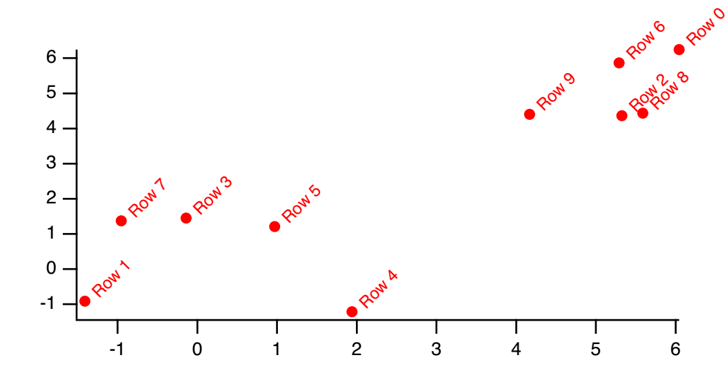
Invoke HCluster to analyze the vectors and create a dendrogram output wave:

HCluster/OTYP=Both vectors

The resulting dendrogram wave, with the default name M_HCluster_Dendrogram, has these contents:

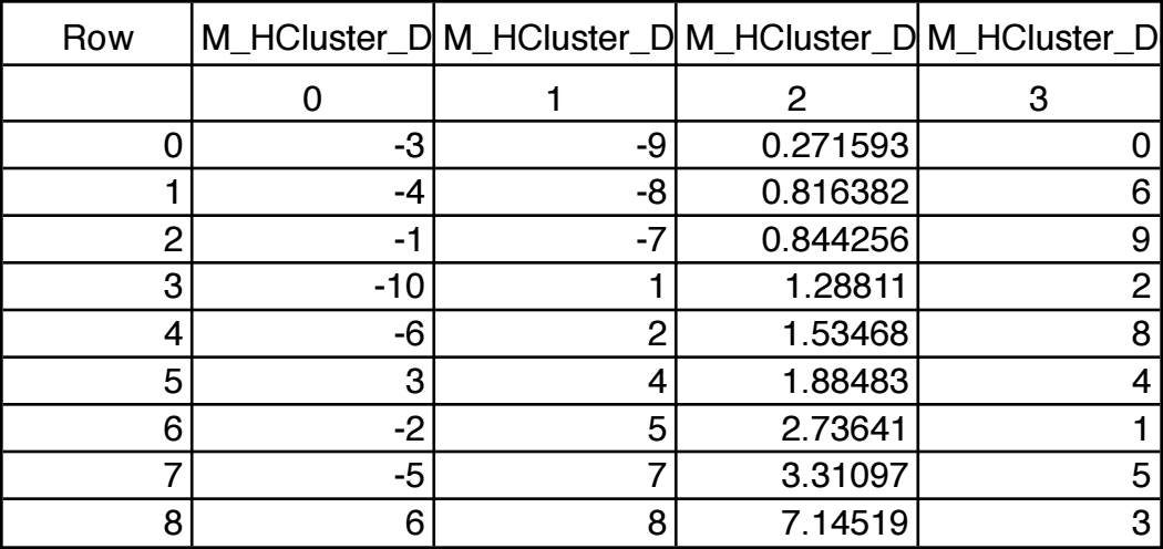
The first row represents the smallest dissimilarity (0.2716). The first two columns indicate that a node has been formed by combining original vector rows 2 and 8 (that is abs(-3)-1 and abs(-9)-1). If we are drawing a dendrogram, we would position rows 2 and 8 at a position 4 and 5 up from the bottom (or down from the top). We see that from the fact that column 3 has row 2 and row 8 listed in those positions. We would draw a tie line between 2 and 8 at a position on the dendrogram proportional to a distance of 0.2716.

The first three rows have negative numbers in columns 0 and 1, showing that they all combine nodes representing the original vectors. If we have text labels for the rows, these nodes would all tie directly to those labels.

Row 3 lists nodes -10 and 1, indicating that it combines an original vector row 9 with the already combined node from row 0 of the dendrogram wave. The relationships between a dendrogram with a heat map of the original vector data, and the dendrogram wave is illustrated here:

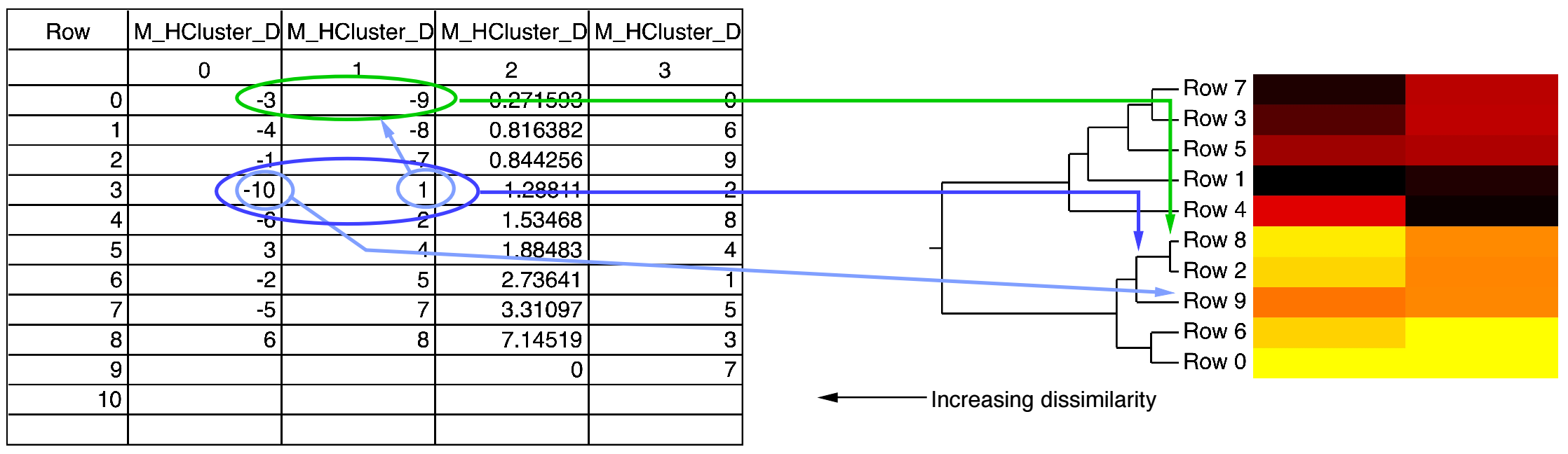
Here we have ordered the vector rows from bottom to top following the ordering given in column 3 of the dendrogram wave. Rows 2 and 8 are tied together with the tie line least distant from the labels. Then Rows 3 and 7 and Rows 0 and 6 are each a bit more distant. Row 3 of the dendrogram wave indicates the tie between the label "Row 9" and the combined node from Row 2 and Row 8.

The two clusters are clearly indicated by the large distance between the most extreme tie line and the next most distant tie line. We might add a "cut line" in that space, and group the two clusters. To show it more clearly, we could color the two clusters differently, possibly like this:

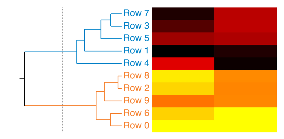
We created this dendrogram with heat map using the Hierarchical Clustering package which you can access by choosing Analysis→Packages→Hierarchical Clustering.

Analysis Programming

This section contains data analysis programming examples. There are many more examples in the WaveMetrics Procedures, Igor Technical Notes, and Examples folders.

Passing Waves to User Functions and Macros

As you look through various examples you will notice two different ways to pass a wave to a function: using a Wave parameter or using a String parameter.

1. Using a Wave Parameter

   Function Test1(w)			
   	Wave w

   • Usable in functions, not in macros.
   • w is a "formal" name. Use it just as if it were the name of an actual wave.
     

2. Using a String Parameter

   Function Test2(wn)
   	String wn

   • Usable in functions and macros.
   • Use the $ operator to convert from a string to a wave name.

The string method is used in macros and in user functions for passing the name of a wave that may not exist but will be created by the called procedure. The wave parameter method is used in user functions when the wave will always exist before the function is called. For details, see Accessing Waves in Functions.

Returning Created Waves from User Functions

A function can return a wave as the function result. For example:

Function Test()
	Wave w = CreateNoiseWave(5, "theNoiseWave")
	WaveStats w
	Display w as "Noise Wave"
End
Function/WAVE CreateNoiseWave(noiseValue, destWaveName)
	Variable noiseValue
	String destWaveName

	Make/O $destWaveName = gnoise(noiseValue)
	Wave w = $destWaveName
	return w
End

If the returned wave is intended for temporary use, you can create it as a free wave:

Function Test()
	Wave w = CreateFreeNoiseWave(5)	// w is a free wave
	WaveStats w
	// w is killed when the function exist
End
Function/WAVE CreateFreeNoiseWave(noiseValue)
	Variable noiseValue

	Make/O/FREE aWave = gnoise(noiseValue)
	return aWave
End

To return multiple waves, you can return a "wave reference wave". See Wave Reference Waves for details.

Writing Functions that Process Waves

The user function is a powerful, general-purpose analysis tool. You can do practically any kind of analysis. However, complex analyses require programming skill and patience.

It is useful to think about an analysis function in terms of its input parameters, its return value and any side effects it may have. By return value, we mean the value that the function directly returns. For example, a function might return a mean or an area or some other characteristic of the input. By side effects, we mean changes that the function causes to any Igor objects. For example, a function might change the values in a wave or create a new wave.

This table shows some of the common types of analysis functions. Examples follow.

Input Parameters	Return Value	Side Effects	Example Function
Source wave	Number	None	WaveSum
Source wave	Not used	Source wave is modifed	RemoveOutliers
Source wave	Wave reference	New output wave is created	LogRatio
Source and destination waves	Not used	Destination wave is modified
Array of wave references	Number	None	WavesMax
Array of wave references	Wave reference	New wave is created	WavesAverage

The following example functions are intended to show you the general form for some common analysis function types. We have tried to make the examples useful while keeping them simple.

WaveSum Example

Input:	Source wave
Return value:	Number
Side effects:	None

// WaveSum(w)
// Returns the sum of the entire wave, just like Igor's sum function.
Function WaveSum(w)
	Wave w

	Variable i, n=numpnts(w), total=0
	for(i=0;i<n;i+=1)
		total += w[i]
	endfor

	return total
End

To use this, you would execute something like

Print "The sum of wave0 is:", WaveSum(wave0)

RemoveOutliers Example

Input:	Source wave
Return value:	Number
Side effects:	Source wave is modified

Often a user function used for number-crunching needs to loop through each point in an input wave. The following example illustrates this.

// RemoveOutliers(theWave, minVal, maxVal)
// Removes all points in the wave below minVal or above maxVal.
// Returns the number of points removed.
Function RemoveOutliers(theWave, minVal, maxVal)
	Wave theWave
	Variable minVal, maxVal

	Variable i, numPoints, numOutliers
	Variable val
	numOutliers = 0
	numPoints = numpnts(theWave)              // number of times to loop

	for (i = 0; i < numPoints; i += 1)
		val = theWave[i]
		if ((val < minVal) || (val > maxVal))  // is this an outlier?
			numOutliers += 1
		else			// if not an outlier
			theWave[i - numOutliers] = val      // copy to input wave
		endif
	endfor

	// Truncate the wave
	DeletePoints numPoints-numOutliers, numOutliers, theWave
	return numOutliers
End

To test this function, try the following commands.

Make/O/N=10 wave0= gnoise(1); Edit wave0
Print RemoveOutliers(wave0, -1, 1), "points removed"

RemoveOutliers uses the for loop to iterate through each point in the input wave. It uses the built-in numpnts function to find the number of iterations required and a local variable as the loop index. This is a very common practice.

The line "if ((val < minVal) || (val > maxVal))" decides whether a particular point is an outlier. || is the logical OR operator. It operates on the logical expressions "(val < minVal)" and "(val > maxVal)". This is discussed in detail under Bitwise and Logical Operators.

To use the WaveMetrics-supplied RemoveOutliers function, include the Remove Points.ipf procedure file:

#include <Remove Points>

See The Include Statement for instructions on including a procedure file.

LogRatio Example

Input:	Source waves
Return value:	Wave reference
Side effects:	Output wave created

// LogRatio(source1, source2, outputWaveName)
// Creates a new wave that is the log of the ratio of input waves.
// Returns a reference to the output wave.
Function/WAVE LogRatio(source1, source2, outputWaveName)
	Wave source1, source2
	String outputWaveName

	Duplicate/O source1, $outputWaveName
	WAVE wOut = $outputWaveName
	wOut = log(source1/source2)
	return wOut
End

To call this from a function, you would execute something like this:

Wave wRatio = LogRatio(wave0, wave1, "ratio")
Display wRatio

The LogRatio function illustrates how to treat input and output waves. Input waves must exist before the function is called and therefore are passed as wave reference parameters. The output wave may or may not already exist when the function is called. If it does not yet exist, it is not possible to create a wave reference for it. Therefore we pass to the function the desired name for the output wave using a string parameter. The function creates or overwrites a wave with that name in the current data folder and returns a reference to the output wave.

WavesMax Example

Input:	Array of wave references
Return value:	Number
Side effects:	None

// WavesMax(waves)
// Returns the maximum value of all waves in the waves array
Function WavesMax(waves)
	Wave/WAVE waves			// A wave containing wave references
	
	Variable theMax = -INF

	Variable numWaves = numpnts(waves)
	Variable i
	for(i=0; i<numWaves; i+=1)
		Wave w = waves[i]
		Variable tmp = WaveMax(w)
		theMax = max(tmp, theMax)
	endfor
	
	return theMax
End

This function shows how you might call WavesMax from another function:

Function DemoWavesMax()
	Make/FREE/N=10 w0 = p
	Make/FREE/N=10 w1 = p + 1
	
	Make/FREE/WAVE waves = {w0, w1}
	
	Variable theMax = WavesMax(waves)
	
	Printf "The maximum value is %g\r", theMax
End

WavesAverage Example

Input:	Array of wave references
Return value:	Wave reference
Side effects:	Creates output wave

// WavesAverage(waves, outputWaveName)
// Returns a reference to a new wave, each point of which contains the
// average of the corresponding points of a number of source waves.
//	waves is assumed to contain at least one wave reference and
// all waves referenced by waves are expected to have the same
// number of points.
Function/WAVE WavesAverage(waves, outputWaveName)
	Wave/WAVE waves         // A wave containing wave references
	String outputWaveName

	// Make output wave based on the first source wave
	Wave first = waves[0]
	Duplicate/O first, $outputWaveName
	Wave wOut = $outputWaveName
	wOut = 0
	
	Variable numWaves = numpnts(waves)
	Variable i
	for(i=0; i<numWaves; i+=1)
		Wave source = waves[i]
		wOut += source       // Add source to output
	endfor

	wOut /= numWaves        // Divide by number of waves

	return wOut
End

This function shows how you might call WavesAverage from another function:

Function DemoWavesAverage()
	Make/FREE/N=10 w0 = p
	Make/FREE/N=10 w1 = p + 1
	
	Make/FREE/WAVE waves = {w0, w1}
	
	Wave wAverage = WavesAverage(waves, "averageOfWaves")
	Display wAverage
End

Finding the Mean of Segments of a Wave

An Igor user who considers each of his waves to consist of a number of segments with some number of points in each segment asked us how he could find the mean of each of these segments. We wrote the FindSegmentMeans function to do this.

Function/WAVE FindSegmentMeans(source, n)
	Wave source
	Variable n     // Number of points in a segment

	String dest    // name of destination wave
	Variable segment, numSegments
	Variable startX, endX, lastX

	dest = NameOfWave(source)+"_m"  	// derive name of dest from source
	numSegments = trunc(numpnts(source)/n)
	if (numSegments < 1)
		DoAlert 0, "Destination must have at least one point"
		return $""  // Null wave reference
	endif

	Make/O/N=(numSegments) $dest
	WAVE destw = $dest

	for (segment = 0; segment < numSegments; segment += 1)
		startX = pnt2x(source, segment*n)            // start X for segment
		endX = pnt2x(source, (segment+1)*n - 1)      // end X for segment
		destw[segment] = mean(source, startX, endX)
	endfor

	return destw
End

This diagram illustrates a source wave with three ten-point segments and a destination wave that will contain the mean of each of the source segments. The FindSegmentMeans function makes the destination wave.

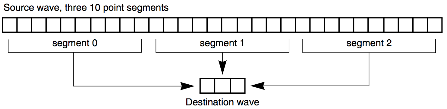
To test FindSegmentMeans, try the following commands.

Make/N=100 wave0=p+1; Edit wave0
FindSegmentMeans(wave0,10)
Append wave0_m

The loop index is the variable "segment". It is the segment number that we are currently working on, and also the number of the point in the destination wave to set.

Using the segment variable, we can compute the range of points in the source wave to work on for the current iteration: segment*n up to (segment+1)*n - 1. Since the mean function takes arguments in terms of a wave's X values, we use the pnt2x function to convert from a point number to an X value.

If it is guaranteed that the number of points in the source wave is an integral multiple of the number of points in a segment, then the function can be speeded up and simplified by using a waveform assignment statement in place of the loop. Here is the statement.

destw = mean(source, pnt2x(source,p*n), pnt2x(source,(p+1)*n-1))

The variable p, which Igor automatically increments as it evaluates successive points in the destination wave, takes on the role of the segment variable used in the loop. Also, the startX, endX and lastX variables are no longer needed.

Using the example shown in the diagram, p would take on the values 0, 1 and 2 as Igor worked on the destination wave. n would have the value 10.

Working with Mismatched Data

Occasionally, you may find yourself with several sets of data each sampled at a slightly different rate or covering a different range of the independent variable (usually time). If all you want to do is create a graph showing the relationship between the data sets then there is no problem.

However, if you want to subtract one from another or do other arithmetic operations then you will need to either:

• Create representations of the data that have matching X values. Although each case is unique, usually you will want to use the Interpolate2 operation (see Using the Interpolate2 Operation) or the interp function (see Using the Interp Function) to create data sets with common X values. You can also use the Resample operation to create a wave to match another.

• Properly set each wave's X scaling, and perform the waveform arithmetic using X scaling values and Igor's automatic linear interpolation. See Mismatched Waves.

The WaveMetrics procedure file Wave Arithmetic Panel uses these techniques to perform a variety of operations on data in waves. You can access the panel by choosing Packages→Wave Arithmetic from the Analysis menu. This will open the procedure file and display the control panel. Click the help button in the panel to learn how to use it.

Analysis References

Brown, P.N., G. D. Byrne, and A. C. Hindmarsh, VODE, a Variable-Coefficient ODE Solver, SIAM J. Sci. Stat. Comput., 10, 1038-1051, 1989.

Cohen, Scott D., and Alan C. Hindmarsh, CVODE User Guide, LLNL Report UCRL-MA-118618, September 1994.

Dennis, J. E., Jr., and Robert B. Schnabel, Numerical Methods for Unconstrained Optimization and Nonlinear Methods, 378 pp., Society for Industrial and Applied Mathematics, Philadelphia, 1996.

Jenkins, M.A., "Algorithm 493, Zeros of a Real Polynomial", ACM Transactions on Mathematical Software, v. 1 no. 2, pp. 178-189, June 1975.

Reinsch, Christian H., Smoothing by Spline Functions, Numerische Mathematic, 10, 177-183, 1967.