Waves

We use the term "wave" to describe the Igor object that contains an array of numbers. Wave is short for "waveform". The main purpose of Igor is to store, analyze, transform and display waves.

Introduction to Igor Pro presents some fundamental ideas about waves. The Guided Tour sections of the Getting Started help file are designed to make you comfortable with these ideas. In this section, we assume that you now have a basic understanding of these concepts.

This section focuses on one-dimensional numeric waves. Waves can have up to four dimensions and can store text data. Multidimensional waves are covered in Multidimensional Waves. Text waves are discussed in this help file.

The primary tools for dealing with waves are Igor's built-in operations and functions and its waveform assignment capability. The built-in operations and functions are described in detail in Igor Pro Reference.

This section covers:

• waves in general
• operations for making, killing and managing waves
• setting and examining wave properties
• waveform assignment

and other topics.

The Waveform Model of Data

A wave consists of a number of components and properties. The most important are:

• the wave name
• the X scaling property
• X units
• an array of data values
• data units

The waveform model of data is based on the premise that there is a straight-line mapping from a point number index to an X value or, stated another way, that the data is uniformly spaced in the X dimension. This is the case for data acquired from many types of scientific and engineering instruments and for mathematically synthesized data. If your data is not uniformly spaced, you can use two waves to form an XY pair. See The XY Model of Data.

A wave is similar to an array in a standard programming language like FORTRAN or C.

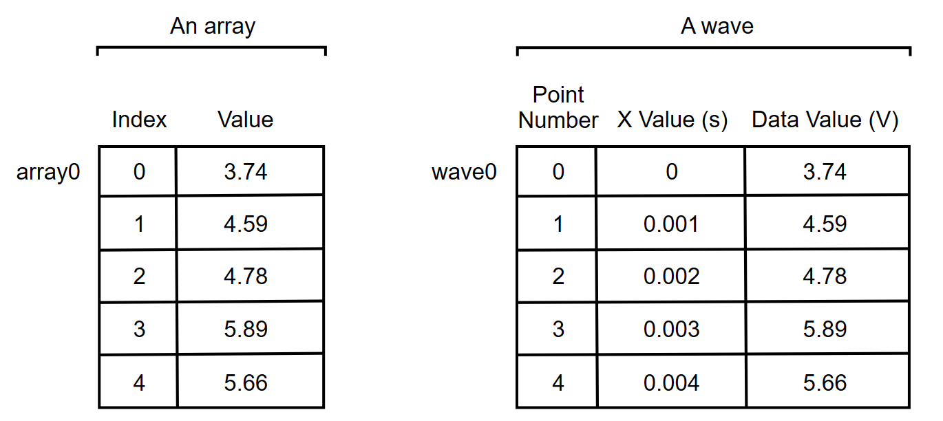
An array in a standard language has a name (array0 in this case) and a number of values. We can reference a particular value using an index.

A wave also has a name (wave0 in this case) and data values. It differs from the array in that it has two indices. The first is called the point number and is identical to an array index or row number. The second is called the X value and is in the natural X units of the data (e.g., seconds, meters). Like point numbers, X values are not stored in memory but rather are computed by Igor.

The X value is related to the point number by the wave's X scaling, which is a property of the wave that you can set. The X scaling of a wave tells Igor how to compute an X value for a given point number using the formula:

x[p] = x0 + p*dx

where x[p] is the X value for point p. The two numbers x0 and dx constitute the wave's X scaling property. x0 is the starting X value. dx is the difference in X value from one point to the next. X values are uniformly spaced along the data's X dimension.

Igor's SetScale operation sets a wave's X scaling. You can use the Change Wave Scaling dialog to generate SetScale commands.

Why does Igor use this model for representing data? We chose this model because it provides all of the information that Igor needs to properly display, analyze and transform waveform data.

By telling Igor your data's X scaling, and X and data units in addition to its data values, you allow Igor to make a proper graph in one step. You can tell Igor to

Display wave0

and it produces a graph like this:

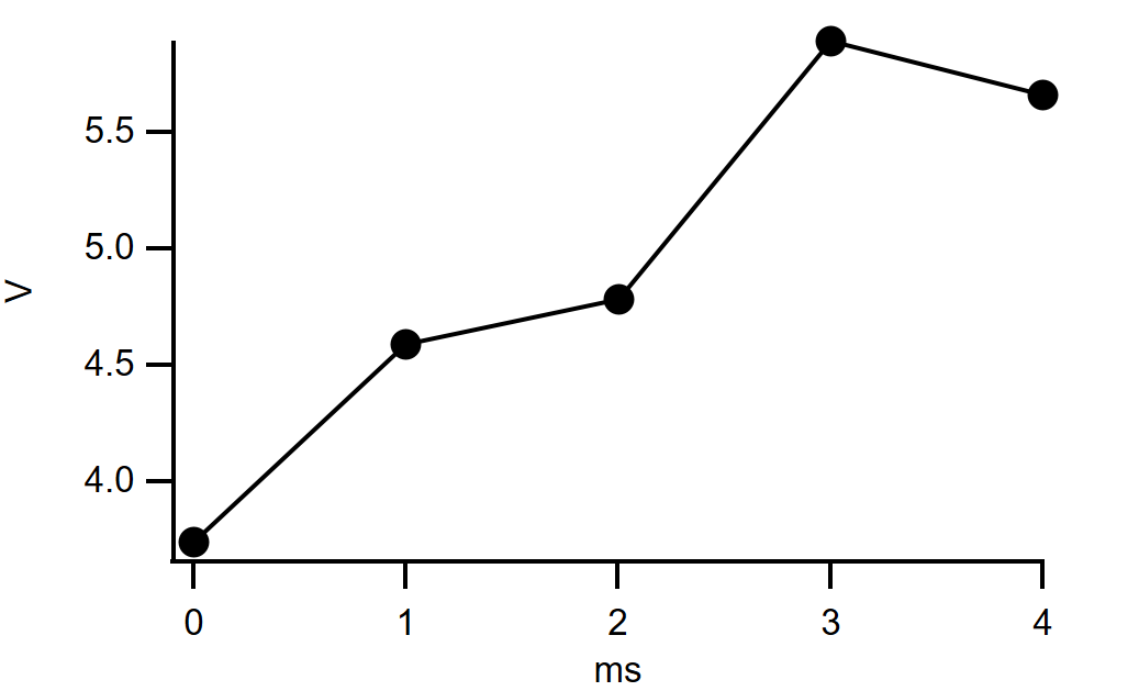
If your data is uniformly spaced on the X axis, it is critical that you understand and use X scaling.

The X scaling information is essential for operations such as integration, differentiation and Fourier transforms and for functions such as the area function. It also simplifies waveform assignment by allowing you to reference a single value or range of values using natural units.

Igor waves can have up to four dimensions. We call these dimensions X, Y, Z and T. X scaling extends to dimension scaling. For each dimension, there is a starting index value (x0, y0, z0, t0) and a delta index value (dx, dy, dz, dt). See Multidimensional Waves for more about multidimensional waves.

The XY Model of Data

If your data is not uniformly spaced along its X dimension then it cannot be represented with a single wave. You need to use two waves as an XY pair.

In an XY pair, the data values of one wave provide X values and the data values of the other wave provide Y values. The X scaling of both waves is irrelevant so we leave it in its default state in which the x0 and dx components are 0 and 1. This gives us

x[p] = 0 + 1*p

This says that a given point's X value is the same as its point number. We call this "point scaling". Here is some sample data that has point scaling.

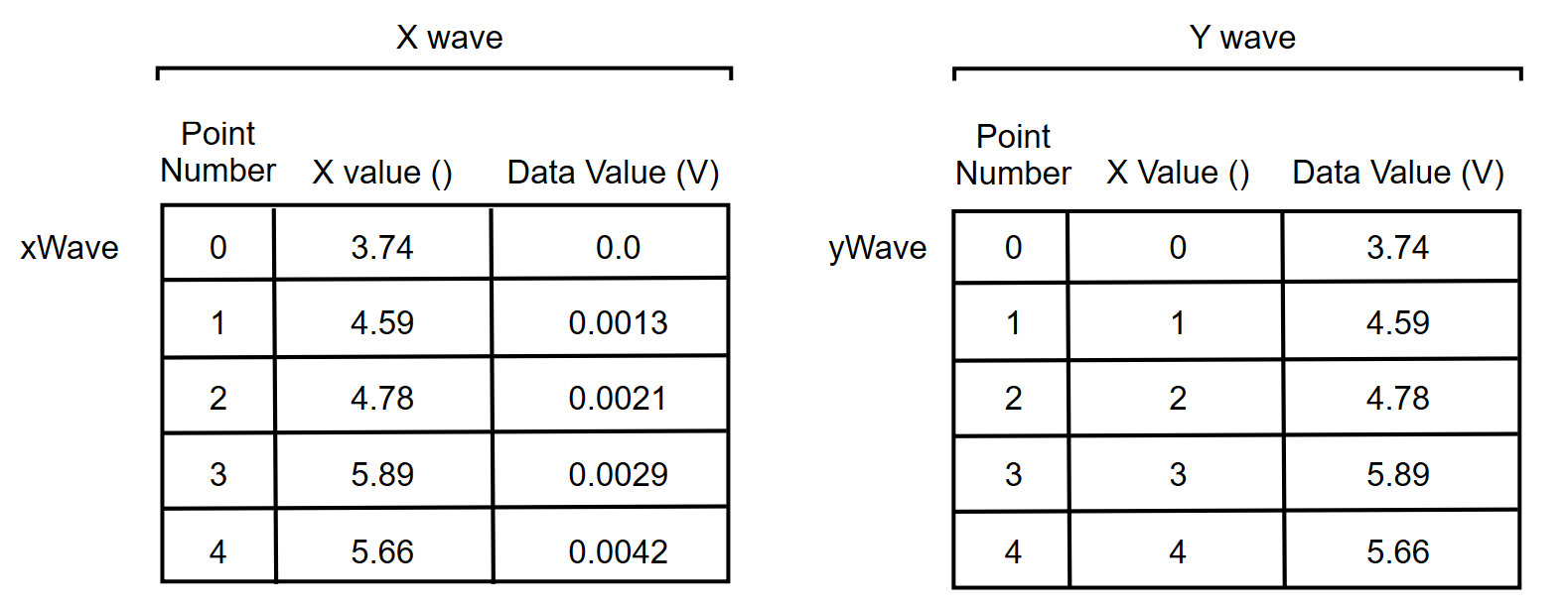
The X values serve no purpose in the XY model. Therefore, we change our thinking and look at an XY pair this way.

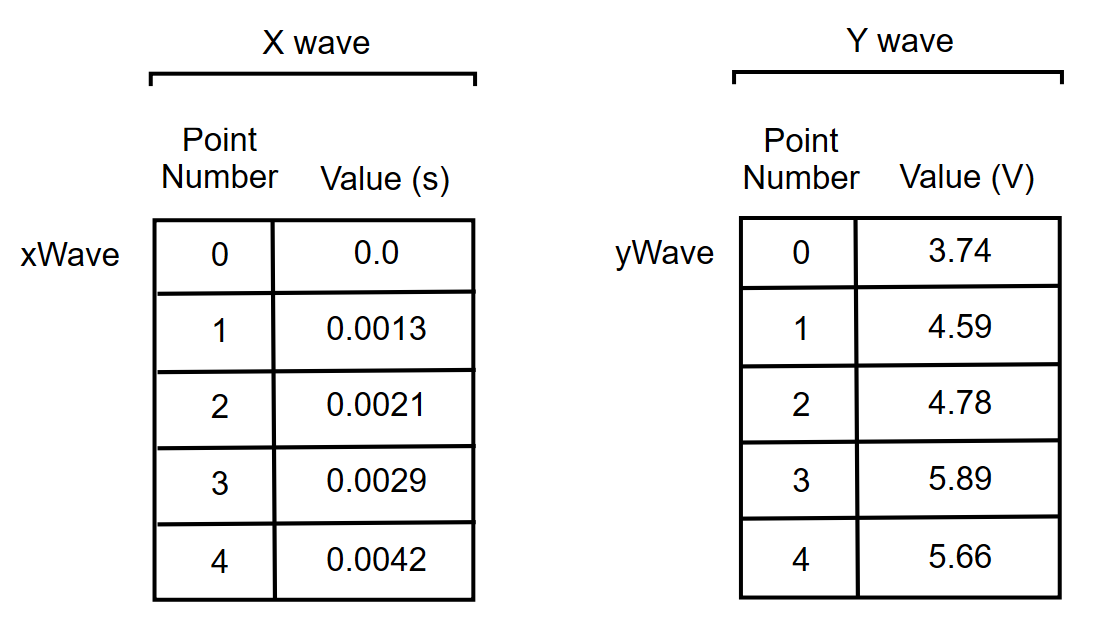
We can tell Igor to

Display yWave vs xWave

and it produces a graph like this.

Some operations, such as Fast Fourier Transforms and convolution, require equally spaced data. In these cases, it may be desirable for you to create a uniformly spaced version of your data by interpolation. See Converting XY Data to a Waveform.

Some people who have uniformly spaced data still use the XY model because it is what they are accustomed to. This is a mistake. If your data is uniformly spaced, it will be well worth your while to learn and use the waveform model. It greatly simplifies graphing and analysis and makes it easier to write Igor procedures.

Making Waves

You can make waves by:

• Loading data from a file
• Typing or pasting in a table
• Using the Make operation (via a dialog or directly from the command line)
• Using the Duplicate operation (via a dialog or directly from the command line)

Most people start by loading data from a file. Igor can load data from text files. In this case, Igor makes a wave for each column of text in the file. Igor can also load data from binary files or application-specific files created by other programs. For information on loading data from files, see Importing Data.

You can enter data manually into a table. This is recommended only if you have a small amount of data. See Using a Table to Create New Waves.

To synthesize data with a mathematical expression, you would start by making a wave using the Make operation. This operation is also often used inside an Igor procedure to make waves for temporary use.

The Duplicate operation is an important and handy tool. Many of Igor's built-in operations transform data in place. Thus, if you want to keep your original data as well as the transformed copy of it, use Duplicate to make a clone of the original.

Wave Names

All waves in Igor have names so that you can reference them from commands. You also use a wave's name to select it from a list or pop-up menu in Igor dialogs or to reference it in a waveform assignment statement.

You need to choose wave names when you use the Make, Duplicate or Rename operations via dialogs, directly from the command line, and when you use the Data Browser.

All names in Igor are case insensitive; wave0 and WAVE0 refer to the same wave.

The rules for the kind of characters that you can use to make a wave name fall into two categories: standard and liberal. Both standard and liberal names are limited to 255 bytes in length.

Prior to Igor Pro 8.00, wave names were limited to 31 bytes. If you use long wave names, your wave and experiment files will require Igor Pro 8.00 or later.

Standard names must start with an alphabetic character (A - Z or a-z) and may contain ASCII alphabetic and numeric characters and the underscore character only. Other characters, including spaces, dashes, periods and non-ASCII characters are not allowed. We put this restriction on standard names so that Igor can identify them unambiguously in commands, including waveform assignment statements.

Liberal names, on the other hand, can contain any character except control characters (such as tab or carriage return) and the following four characters:

"	'	:	;

Standard names can be used without quotation in commands and expressions but liberal names must be quoted. For example:

Make wave0; wave0 = p               // wave0 is a standard name
Make 'wave 0'; 'wave 0' = p         // 'wave 0' is a liberal name

Igor cannot unambiguously identify liberal names in commands unless they are quoted. For example, in

wave0 = miles/hour

miles/hour could be a single wave or it could be the quotient of two waves.

To make them unambiguous, you must enclose liberal names in single straight quotes whenever they are used in commands or waveform arithmetic expressions. For example:

wave0 = 'miles/hour'
Display 'run 98', 'run 99'

note

Writing procedures that work with liberal names requires extra effort and testing on the part of Igor programmers (see Programming with Liberal Names). We recommend that you avoid using liberal names until you understand the potential problems and how to solve them.

See Object Names for a discussion of object names in general.

Number of Dimensions

Waves can consist of one to four dimensions. You determine this when you make a wave. You can change it using the Redimension operation. See Multidimensional Waves for details.

Wave Data Types

Each wave has a data type that determines the kind of data that it stores. You set a wave's data type when you make it. You can change it using the Data Browser, the Redimension operation or the Redimension dialog.

There are three classes of wave data types:

• Numeric data types
• Text
• References (wave references and data folder references)

Each numeric data type can be either real or complex. Text and reference data types cannot be complex.

Reference data types are used in programming only.

You can programmatically determine the data type of a wave using the WaveType function.

Numeric Wave Data Types

This table shows the numeric wave data types available in Igor.

Data Type	Range	Bytes per point
Double-precision	floating point ≅15 decimal digits	8
Single-precision	floating point ≅7 decimal digits	4
Signed 64-bit integer	-2^63 to 2^63 - 1	8
Signed 32-bit integer	-2,147,483,647 to 2,147,483,648	4
Signed 16-bit integer	-32,768 to 32,767	2
Signed 8-bit integer	-128 to 127	1
Unsigned 64-bit integer	0 to 2^64 - 1	8
Unsigned 32-bit integer	0 to 4,294,967,295	4
Unsigned 16-bit integer	0 to 65,535	2
Unsigned 8-bit integer	0 to 255	1

The 64-bit integer types were added in Igor Pro 7.00.

For most work, single precision waves are appropriate.

Single precision waves take up half the memory and disk space of double precision. With the exception of the FFT and some special purpose operations, Igor uses double precision for calculations regardless of the numeric precision of the source wave. However, the narrower dynamic range and smaller precision of single precision is not appropriate for all data. If you are not familiar with numeric errors due to limited range and precision, it is safer to use double precision for analysis.

Integer waves are intended for data acquisition purposes and are not intended for use in analysis. See Integer Waves for details.

Default Wave Properties

When you create a wave using the Make operation with no optional flags, it has the following default properties.

Property	Default
Number of points	128
Data type	Real, single-precision floating point
X scaling	x0=0, dx=1 (point scaling)
X units	Blank
Data units	Blank

These are the key wave properties. For a comprehensive list of properties, see Wave Properties.

If you make a wave by loading it from a file or by typing in a table, it has the same default properties except for the number of points.

However you make waves, if they represent waveforms as opposed to XY pairs, you should use the Change Wave Scaling dialog to set their X scaling and units.

Make Operation

Most of the time you will probably make waves by loading data from a file (see Importing Data), by entering it in a table (see Using a Table to Create New Waves), or by duplicating existing waves (see The Duplicate Operation).

The Make operation is used for making new waves. See the Make operation for additional details.

Here are some reasons to use Make:

• To make waves to play around with.

• For plotting mathematical functions.

• To hold the output of analysis operations.

• To hold miscellaneous data, such as the parameters used in a curve fit or temporary results within an Igor procedure.

The Make Waves dialog provides an interface to the Make operation. To use it, choose Make Waves from the Data menu.

Waves have a definite number of points. Unlike a spreadsheet program which automatically ignores blank cells at the end of a column, there is no such thing as an "unused point" in Igor. You can change the number of points in a wave using the Redimension Waves Dialog or the Redimension operation.

The "Overwrite existing waves" option is useful when you don't know or care if there is a wave with the same name as the one you are about to make.

Make Operation Examples

Make coefs for use in curve fitting:

Make/O coefs = {1.5, 2e-3, .01}

Make a wave for plotting a math function:

Make/O/N=200 test; SetScale x 0, 2*PI, test; test = sin(x)

Make a 2D wave for image or contour plotting:

Make/O/N=(20,20) w2D; w2D = (p-10)*(q-10)

Make a text wave for a category plot:

Make/O/T quarters = {"Q1", "Q2", "Q3", "Q4"}

It is often useful to make a clone of an existing wave. Don't use Make for this. Instead use the Duplicate operation.

Make/O does not preserve the contents of a wave and in fact will leave garbage in the wave if you change the number of points, numeric precision or numeric type. Therefore, after doing a Make/O you should not assume anything about the wave's contents. If you know that a wave exists, you can use the Redimension operation instead of Make. Redimension does preserve the wave's contents.

Waves and the Miscellaneous Settings Dialog

The state of the Type popup in the Make Waves dialog, the precision of waves created by typing in a table, and the way Igor Binary waves are loaded (whether they are copied or shared) are preset with the Miscellaneous Settings dialog using the Data Loading Settings category.

Changing Dimension and Data Scaling

When you make a 1D wave, it has default X scaling, X units and data units. You should use the SetScale operation to change these properties.

The Change Wave Scaling dialog provides an interface to the SetScale operation. To use it, choose Change Wave Scaling from the Data menu.

Scaled dimension indices can represent ordinary numbers, dates, times or date&time values. In the most common case, they represent ordinary numbers and you can leave the Units Type pop-up menu in the Set X Properties section of the dialog on its default value: Numeric.

If your data is waveform data, you should enter the appropriate Start and Delta X values. If your data is XY data, you should enter 0 for Start and 1 for Delta. This results in the default "point scaling" in which the X value for a point is the same as the point number.

Normally you should leave the Set X Properties and Set Data Properties checkboxes selected. Deselect one of them if you want the dialog to generate commands to set only X or only Data properties. When working with multidimensional data, the X of Set X Properties can be changed to Y, Z or T via the pop-up menu. See Multidimensional Waves.

If you want to observe the properties of a particular wave, double-click it in the list or select the wave and then click the From Wave button. This sets all of the dialog items according to that wave's properties.

Igor uses the dimension and data Units to automatically label axes in graphs. Igor can handle units consisting of 49 bytes or less. Typically, units should be short, standard abbreviations such as "m", "s", or "g". If your data has more complex units, you can enter the complex units or you may prefer to leave the units blank.

Advanced Dimension and Data Scaling

If you click More Options, Igor displays some additional items in the dialog. They give you two additional ways to specify X scaling and allow you to set the wave's "data full scale" values. These options are usually not needed but for completeness are described in this section.

In spite of the fact that there is only one way of calculating X values, there are three ways you can specify the x0 and dx values. Use the SetScale Mode pop-up menu to change the meaning of the scaling entries above. The simplest way is to simply specify x0 and dx directly. This is the Start and Delta mode in the dialog and is the only way of setting the scaling unless you click the More Options button. As an example, if you have data that was acquired by a digitizer that was set to sample at 1 MHz starting 150 µs after t=0, you would enter 150E-6 for Start and 1E-6 for Delta.

The other two ways of specifying X scaling are to tell Igor what the starting and ending X values are and allow Igor to calculate dx from the number of points. In the Start and End mode you specify the X value of the last data point. Using the Start and Right mode you specify the X at the end of the last interval. For example, assuming our digitizer (above) created a 100 point wave, we would enter 150E-6 as Start for either mode. If we selected the Start and End mode we would enter 249E-6 for End (150E-6 + 99*1E-6). If we selected Start and Right we would enter 250E-6 for Right.

The min and max entries allow you to set a property of a wave called its "data full scale". This property doesn't serve a critical purpose. Igor does not use it for any computation or graphing purposes. It is merely a way for you to document the conditions under which the wave data was acquired. For example, if your data comes from a digital oscilloscope and was acquired on the ±10v range, you could enter -10 for min and +10 for max. When you make waves, both of these will initially be set to zero. If your data has a meaningful data full scale, you can set them appropriately. Otherwise, leave them zero.

The data units, on the other hand are used for graphing purposes, just like the dimension units.

Date, Time, and Date&Time Units

The units "dat" are special. They tell Igor that the scaled dimension indices or data values of a wave contain date, time, or date&time information.

If you have waveform data then set the X units of your waveform to "dat".

If you have XY data then set the data units of your X wave to "dat". In this case your X wave must be double-precision floating point in order to have enough precision to represent dates accurately.

For example, if you have a waveform that contains some quantity measured once per day, you would set the X units for the wave to "dat", set the starting X value to the date on which the first measurement was done, and set the Delta X value to one day. Choosing Date from the Units Type pop-up menu sets the X units to "dat". You can enter the starting value as a date rather than as a number of seconds since 1/1/1904, which is how Igor represents dates internally. When Igor graphs the waveform, it will notice that the X units are "dat" and will display dates on the X axis.

If instead of a waveform, you have an XY pair, you would set the data units of the X wave to "dat", by choosing Date from the Units Type pop-up menu in the Set Data Properties section of the dialog. When you graph the XY pair, Igor will notice that the X wave contains dates and will display dates on the X axis.

The Units Type pop-up menus do not correspond directly to any property of a wave. That is, a wave doesn't have a units type property. Instead, these menus merely tell Igor what kind of values you are dealing with so that the dialog can display the values in the appropriate format.

For further discussion of how Igor represents dates, see Date/Time Waves.

For information on dates and times in tables, see Date/Time Formats.

For information on dates and times in graphs, see Date/Time Axes.

The Duplicate Operation

Duplicate is a handy and frequently-used operation. It can make new waves that are exact clones of existing waves. It can also clone a section of a wave and thus provides an easy way to break a big wave up into smaller waves.

Here are some reasons to use Duplicate:

• To hold the results of a transformation (e.g. integration, differentiation, FFT) while preserving the original data.

• To hold the "destination" of a curve fit.

• For holding temporary results within an Igor procedure.

• To extract a section of a wave.

The Duplicate Waves dialog provides an interface to the Duplicate operation. To use it, choose Duplicate Waves from the Data menu.

The cursors button is used in conjunction with a graph. You can make a graph of your template wave. Then put the cursors on the section of the template that you want to extract. Choose Duplicate Waves from the Data menu and click the cursors button. Then click Do It. This clones the section of the template wave identified by the cursors.

People sometimes make the mistake of using the Make operation when they should be using Duplicate. For example, the destination wave in a curve fit must have the same number of points, numeric type and numeric precision as the source wave. Duplicating the source wave insures that this will be true.

Duplicate Operation Examples

Clone a wave and then transform the clone:

Duplicate/O wave0, wave0_d1; Differentiate wave0_d1

Use Duplicate to inherit the properties of the template wave:

Make/N=200 wave0; SetScale x 0, 2*PI, wave0; wave0 = sin(x)
Duplicate wave0, wave1; wave1 = cos(x)

Make a destination wave for a curve fit:

Duplicate/O data1, data1_fit
CurveFit gauss data1 /D=data1_fit

Compare the first half of a wave to the second:

Duplicate/O/R=[0,99] data1, data1_1
Duplicate/O/R=[100,199] data1, data1_2
Display data1_1, data1_2

We often use the /O flag (overwrite) with Duplicate because we don't know or care if a wave already exists with the new wave name.

Killing Waves

The KillWaves operation removes waves from the current experiment. This releases the memory used by the waves. Waves that you no longer need clutter up lists and pop-up menus in dialogs. By killing them, you reduce this clutter.

Here are some situations in which you would use KillWaves:

• You are finished examining data that you loaded from a file.

• You are finished using a wave that you created for experimentation.

• You no longer need a wave that you created for temporary use in an Igor procedure.

The Kill Waves dialog provides an interface to the KillWaves operation. To use it, choose Kill Waves from the Data menu.

Igor will not let you kill waves that are used in graphs, tables or user-defined functions so they do not appear in the list.

note

Igor cannot tell if a wave is referenced from a macro. Thus, Igor will let you kill a wave that is referenced from a macro but not used in any other way. The most common case of this is when you close a graph and save it as a recreation macro. Waves that were used in the graph are now used only in the macro and Igor will let you kill them. If you execute the graph recreation macro, it will be unable to recreate the graph.

KillWaves can delete the Igor binary wave file from which a wave was loaded, called the "source file". This is normally not necessary because the wave you are killing either has never been saved to disk or was saved as part of a packed experiment file and therefore was not loaded from a standalone file.

The "Kill all waves not in use" option is intended for those situations where you have created an Igor experiment that contains procedures which load, graph and process a batch of waves. After you have processed one batch of waves, you can kill all graphs and tables and then kill all waves in the experiment in preparation for loading the next batch. This affects only those waves in the current data folder; waves in any other data folders will not be killed.

KillWaves Operation Examples

Here are some simple examples using KillWaves.

// Kills all target windows and all waves.
// Does not kill nontarget windows (procedure and help windows).
Function KillEverything()
   String windowName
	
   do
      windowName = WinName(0, 1+2+4+16+64)   // Get next target window
      if (CmpStr(windowName, "") == 0)       // If name is ""
         break                               // we are done so break loop
      endif
      KillWindow $windowName                 // Kill this target window
   while (1)
	
   KillWaves/A                               // Kill all waves
End

// This illustrates killing a wave used temporarily in a procedure
Function Median(w)                           // Returns median value of wave w
   Wave w

   Variable result

   Duplicate/O w, temp                       // Make a clone of wave
   Sort temp, temp                           // Sort clone
   result = temp[numpnts(temp)/2]

   KillWaves temp                            // Kill clone

   return result
End

For more examples, see the "Kill Waves" procedure file in the "WaveMetrics Procedures" folder.

Browsing Waves

The Data Browser (Data menu) lets you see what waves (as well as strings and variables) exist at any given time. It also lets you see what data folders exist and set the current data folder. The Data Browser is described in detail in Data Folders.

Igor Pro 6 had a Browse Waves dialog which you accessed via Data->Browse Waves. Because the dialog provided the same functionality as the Data Browser, the dialog and menu item were removed in Igor Pro 7.00.

Renaming Waves

You can rename a wave using:

• The Data Browser

• The Rename dialog (Data menu)

• The Rename operation from the command line

The Rename operation renames waves as well as other objects.

Here are some reasons for renaming waves:

• You have loaded a bunch of waves from a file and Igor auto-named the waves.

• You have decided on a naming convention for waves and you want to make existing waves follow the convention.

• You are about to load a set of waves whose names will be the same as existing waves and you want to get the existing waves out of the way but still keep them in memory. (You could also achieve this by moving them to a new data folder.)

To use the Rename operation, choose Rename from the Data menu. This brings up the Rename Objects dialog.

Redimensioning Waves

The Redimension operation can change the following properties of a wave:

• The number of dimensions in the wave

• The number of elements in each dimension

• The numeric precision (e.g., single to double)

• The numeric type (e.g., real to complex)

The Redimension Waves dialog provides an interface to the Redimension operation. To use it, choose Redimension Waves from the Data menu.

When Redimension adds new elements to a wave, it sets them to zero for a numeric wave and to blank for a text wave.

The following commands illustrate two ways of changing the numeric precision of a wave. Redimension preserves the contents of the wave whereas Make does not.

Make/N=5 wave0=x
Edit wave0
Redimension/D wave0     // This preserves the contents of wave0
Make/O/D/N=5 wave0      // This does not

See Vector (Waveform) to Matrix Conversion for information on converting a 1D wave into a 2D wave while retaining the data (i.e., reshaping).

Igor does not allow you to change a wave from numeric to text or vice versa. The following examples illustrate how you can make a text copy of a numeric wave and a numeric copy of a text wave:

Make/N=10 numWave = p
Make/T/N=(numpnts(numWave)) textWave = num2str(numWave)
Make/N=(numpnts(textWave)) numWave2 = str2num(textWave)

However, you can lose precision because num2str prints with only 6 digits of precision.

Inserting Points

There are two ways to insert new points in a wave. You can do this by:

• Using the InsertPoints operation

• Typing or pasting in a table

This section deals with the InsertPoints operation. For information on typing or pasting in a table, see Tables.

Using the InsertPoints operation, you can insert new data points at the start, in the middle or at the end of a 1D wave. You can also insert new elements in multidimensional waves. For example, you can insert new columns in a 2D matrix wave. The inserted values will be 0 for a numeric wave and "" for a text wave.

The Insert Points dialog provides an interface to the InsertPoints operation. To use it, choose Insert Points from the Data menu.

If the value that you enter for first point is greater than the number of elements in the selected dimension of a selected wave, the new points are added at the end of the dimension. InsertPoints can change the dimensionality of a wave. For example, if you insert a column in a 1D wave, you end up with at 2D wave.

If the top window is a table at the time that you select Insert Points, Igor will preset the dialog items based on the selection in the table.

Deleting Points

There are two ways to delete points from a wave. You can do this by:

• Using the DeletePoints operation

• Doing a cut in a table

This section deals with the DeletePoints operation. For information on cutting in a table, see Tables.

Using the DeletePoints operation, you can delete data points from the start, middle or end of a 1D wave. You can also delete elements from multidimensional waves. For example, you can delete columns from a 2D matrix wave.

The Delete Points dialog provides an interface to the DeletePoints operation. To use it, choose Delete Points from the Data menu.

If the value that you enter for first point is greater than the number of elements in the selected dimension of a selected wave, DeletePoints will do nothing to that wave. If the number of elements is too large, DeletePoints will delete from the specified first element to the end of the dimension.

Except for the case of removing all elements, which leaves the wave as 1D, DeletePoints does not change the dimensionality of a wave. Use Redimension for that.

If the top window is a table at the time that you choose Delete Points, Igor will preset the dialog items based on the selection in the table.

Waveform Arithmetic and Assignment

Waveform arithmetic is a very flexible and powerful part of Igor's analysis capability. You can write assignment statements that work on an entire wave or on a subset of a wave, much as you would write an assignment to a single variable in a standard programming language.

In a wave assignment statement, a wave appears on the left side and a mathematical expression appears on the right side. Here are some examples.

wave0 = sin(x)
wave0 = log(wave1/wave2)
wave0[0,99] = wave1[100 + p]

A wave on the left side is called the destination wave. A wave on the right side is called a source wave.

When Igor executes a wave assignment statement, it evaluates the expression on the right-hand side one time for each point in the destination wave. The result of each evaluation is stored in the corresponding point in the destination wave.

During execution, the symbol p has a value equal to the number of the point in the destination wave which is being set and the symbol x has a value equal to the X value at that point. The X value for a given point is determined by the number of the point and the X scaling for the wave. To see this, execute the following commands, one-at-a-time:

Make/N=5 wave0; SetScale/P x 0, .1, wave0; Edit wave0.xy
wave0 = p
wave0 = x

The first assignment statement sets the value of each point of wave0 to the point number. The second assignment statement sets the value of each point of wave0 to the X value for that point.

A source wave returns its data value at the point being evaluated. In the example

wave0 = log(wave1/wave2)

Igor evaluates the right-hand expression once for each point in wave0. During each evaluation of the expression, wave1 and wave2 return their data values at the point being evaluated. Consequently, these commands are equivalent:

wave0 = log(wave1/wave2)
wave0 = log(wave1[p]/wave2[p])

Understanding Wave Assignments

To understand wave assignments, it is critical to understand the meaning of p and x. To this end, it may be helpful to think of what happens inside Igor. A wave assignment statement causes a loop to run inside Igor.

p is the loop index of the internal loop and runs over the range of points being set in the destination wave. In the preceding example, p starts from 0 and is incremented each time through the internal loop, up to N-1, where N is the number of points in wave0. For each value of p, the right-hand expression is evaluated and the result is stored in the corresponding point of wave0.

When you see wave1 or wave1[p] on the right-hand side of a waveform assignment statement, this returns the value of wave1 at point p, which is the point in the destination wave (wave0) that Igor is setting during the current iteration of the internal loop.

x is similar to p except that, instead of being the loop index of the Igor internal loop, it is calculated from the loop index using the X scaling of the destination wave:

x = x0 + p*dx

Wave assignment is an important Igor feature and it will be worth your time to understand it. You may need to reread this material and do some experimentation on the command line. If you are new to Igor, you may prefer to return to this topic after you have gained experience.

Wave Assignment Example

This command sequence illustrates some of the ideas explained above.

Make/N=200 wave1, wave2                // Two waves, 200 points each
SetScale/P x, 0, .05, wave1, wave2     // Set X values from 0 to 10
Display wave1, wave2                   // Create a graph of waves
wave1 = sin(x)                         // Assign values to wave1
wave2 = wave1 * exp(-x/5)              // Assign values to wave2

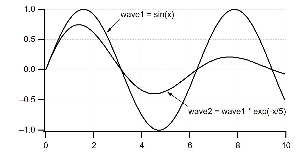
Since wave1 has 200 points, the wave assignment statement wave1=sin(x) evaluates sin(x) 200 times, once for each point in wave1. The first point of wave1 is point number 0 and the last point of wave1 is point number 199. The symbol p, not used in this example, goes from 0 to 199. The symbol x steps through the 200 X values for wave1 which start from 0 and step by .05, as specified by the SetScale command. The result of each evaluation is stored in the corresponding point in wave1, making wave1 about 1.5 cycles of a sine wave.

Since wave2 also has 200 points, the wave assignment statement wave2=wave1exp(-x/5) evaluates wave1exp(-x/5) 200 times, once for each point in wave2. In this assignment, the right-hand expression contains a wave, wave1. As Igor executes the assignment, p goes from 0 to 199. Each of the 200 times the right side is evaluated, wave1 returns its data value for the corresponding point. The result of each evaluation is stored in the corresponding point in wave2 making wave2 about 1.5 cycles of a damped sine wave.

The effect of a wave assignment statement is to set the data values of the destination wave. Igor does not remember the functional relationship implied by the assignment. In this example, if you changed wave1, wave2 would not change automatically. If you wanted wave2 to have the same functional relationship to wave1 as it had before you changed wave1, you would have to reexecute the wave2=wave1*exp(-x/5) assignment.

There is a special kind of wave assignment statement that does establish a functional relationship. It should be used sparingly. See Wave Dependency Formulas for details.

More Wave Assignment Features

Just as the symbol p returns the current element number in the rows dimension, the symbols q, r and s return the current element number in the columns, layers and chunks dimensions of multidimensional waves. The symbol x in the rows dimension has analogs y, z and t in the columns, layers and chunks dimensions. See Multidimensional Waves, for details.

You can use multiple processors to execute a waveform assignment statement that takes a long time. See Automatic Parallel Processing with Multithread for details.

The right-hand expression is evaluated in the context of the data folder containing the destination wave. See Data Folders and Assignment Statements for details.

Usually source waves have the same number of points and X scaling as the destination wave. In some cases, it is useful to write a wave assignment statement where this is not true. This is discussed under Mismatched Waves.

Indexing and Subranges

Igor provides two ways to refer to a specific point or range of points in a 1D wave: X value indexing and point number indexing. Consider the following examples.

wave0[54] = 92       // Sets wave0 at point 54 to 92
wave0(54) = 92       // Sets wave0 at X=54 to 92
wave0[1,10] = 92     // Sets wave0 from point 1 to point 10 to 92
wave0(1,10) = 92     // Sets wave0 from X=1 to X=10 to 92

Brackets tell Igor that you are indexing the wave using point numbers. The number or numbers inside the brackets are interpreted as point numbers of the indexed wave.

Parentheses tell Igor that you are indexing the wave using X values. The number or numbers inside the parentheses are interpreted as X values of the indexed wave. When you use an X value as an index, Igor first finds the point number corresponding to that X value based on the indexed wave's X scaling, and then uses that point number as the point index.

If the wave has point scaling then these two methods have identical effects. However, if you set the X scaling of the wave to other than point scaling then these commands behave differently. In both cases the range is inclusive.

You can specify not only a range but also a point number increment. For example:

wave0[0,98;2] = 1    // Sets even numbered points in wave0 to 1
wave0[1,99;2] = -1   // Sets odd numbered points in wave0 to -1

The number after the semicolon is the increment. Igor begins at the starting point number and goes up to and including the ending point number, skipping by the increment. At each resulting point number, it evaluates the right-hand side of the wave assignment statement and sets the destination point accordingly.

Increments can also be used when you specify a range in terms of X value but the increment is always in terms of point number. For example:

wave0(0,100;5) = PI  // Sets wave0 at specified X values to PI

Here Igor starts from the point number corresponding to x = 0 and goes up to and including the point number that corresponds to x = 100. The point number is incremented by 5 at each iteration.

You can take some shortcuts in specifying the range of a destination wave. The subrange start and end values can both be omitted. When the start is omitted, point number zero is used. When the end is omitted, the last point of the wave is used. You can also use a * character or INF to specify the last point. An omitted increment value defaults to a single point.

Here are some examples that illustrate these shortcuts:

wave0[ ,50] = 13     // Sets wave0 from point 0 to point 50
wave0[51,] = 27      // Sets wave0 from point 51 to last point
wave0[51,*] = 27     // Sets wave0 from point 51 to last point
wave0[51,INF] = 27   // Sets wave0 from point 51 to last point
wave0[ , ;2] = 18.7  // Sets every even point of wave0
wave0[1,*;2] = 100   // Sets every odd point of wave0

A subrange of a destination wave may consist of a single point or a range of points but a subrange of a source wave must consist of a single point. In other words the wave assignment statement:

wave1(4,5) = wave2(5,6)    // Illegal!

is not legal. In this assignment, x ranges from 4 to 5. You can get the desired effect using:

wave1(4,5) = wave2(x+1)    // OK!

By virtue of the range specified on the left hand side, x goes from 4 to 5. Therefore, x+1 goes from 5 to 6 and the right-hand expression returns the values of wave2 from 5 to 6.

Indexing With an Index Wave

You can set specific elements of the destination wave using another wave to provide index values using this syntax:

destWave[indexWave] = <expression>

This feature was added in Igor Pro 8.00.

When the destination wave is one dimensional, the index wave must contain a list of valid point numbers. For example:

Make/O/N=10 destWave = 0
Make/O indexWave = {2,5,8}
destWave[indexWave] = p; Print destWave
	destWave[0]= {0,0,2,0,0,5,0,0,8,0}

When the destination wave is multidimensional, the index wave can be two dimensional with a valid row index in the first column and a valid column index in the second column. The next example sets all elements of the destination wave to zero except for elements (3,2), (5,4), and (7,6) which it sets to 999.

Make/O/N=(10,10) destWave = 0
Make/O/N=(3,2) indexWave
indexWave[0][0] = {3,5,7}     // Store row indices in column 0
indexWave[0][1] = {2,4,6}     // Store column indices in column 1
Edit indexWave
destWave[indexWave] = 999
Edit destWave

When the destination wave is multidimensional, it is legal for the index wave to be 1D containing linear point numbers as if the destination wave were itself 1D. The assignment statement is evaluated as if the destination wave were 1D so q, r, s, y, z and t return zero on the righthand side. This example uses a 1D index wave to set the same elements as the preceding example:

Make/O/N=(10,10) destWave = 0
Make/O indexWave = {23,45,67}
destWave[indexWave] = 888

In addition to using an index wave on the left hand side, you can also use a value wave on the right with this syntax:

destWave[indexWave] = {valueWave}

The value wave is a 1D vector of values. It should contain the same number of values as there are index values and should have the same type (numeric, string, etc.) as the destination wave. Here is an example:

Make/O/N=10 destWave = 0
Make/O indexWave = {2,5,8}
Make/O valueWave = {777,776,775}
destWave[indexWave] = {valueWave}

When you use an index wave, a list of individual values is not supported:

destWave[indexWave] = {777,776,775}    // Error - value wave expected in braces

In the next example we treat a 2D destination wave as 1D by providing a 1D index wave:

Make/O/N=(10,10) destWave = 0
Make/O indexWave = {23,45,67}
Make/O valueWave = {666,665,664}
destWave[indexWave] = {valueWave}

In the next example we treat a 2D the destination wave as 2D by providing a 2D index wave:

Make/O/N=(10,10) destWave = 0
Make/O/N=(3,2) indexWave
indexWave[0][0] = {3,5,7}        // Store row indices in column 0
indexWave[0][1] = {2,4,6}        // Store column indices in column 1
Make/O valueWave = {555,554,553}
destWave[indexWave] = {valueWave}

Interpolation in Wave Assignments

If you specify a fractional point number or an X value that falls between two data points, Igor will return a linearly interpolated data value. For example, wave1[1.75] returns the value of wave1 three-quarters of the way from the data value of point 1 to the data value of point 2. This interpolation is done only for one-dimensional waves. See Multidimensional Wave Assignment, for information on assignments with multidimensional data.

This is a powerful feature. Imagine that you have an evenly spaced calibration curve, called calibration, and you want to find the calibration values at a specific set of X coordinates as stored in a wave called xData. If you have set the X scaling of the calibration wave, you can do the following:

Duplicate xData, yData
yData = calibration(xData)

This uses the interpolation feature of Igor's wave assignment statement to find a linearly-interpolated value in the calibration wave for each X coordinate in the xData wave.

Lists of Values

You can assign values to a wave or to a subrange of a wave using a list of values in curly braces. You can also add rows and columns.

1D Lists of Values

This section shows how to set elements of a 1D wave and add rows using lists of values. As shown below a 1D list of values consists of a lists of row values in curly braces.

Make/O/N=5 wave0 = NaN     // Make 5 point wave and display in table
Edit/W=(5,45,450,350) wave0

wave0 = {0, 1, 2}          // Redimension wave0 to 3 rows and set Y values to 0, 1, 2

Make/O/N=5 wave0 = NaN     // Restore to 5 points

wave0[1,3]= {1, 2, 3}      // Set points 1 through 3 to 1, 2, 3

wave0 = NaN
wave0[1]= {1, 2, 3}        // Set points 1 through 3 to 1, 2, 3 (same as previous example)

wave0 = NaN
wave0[0,4;2]= {0, 2, 4}    // Set points 0, 2, and 4 to 0, 2, 4 using a step size of 2

// Extend wave0 from 5 rows to 8 rows and set new Y values.
// Adds rows because the index, 5, is equal to the number of wave rows.
wave0 = NaN
wave0[5]= {5, 6, 7}

Make/O/N=5 wave0 = NaN     // Restore to 5 points

// Add a column changing wave0 from 1D to 2D.
// Adds a column because the column index, 1, is equal to the number of wave columns.
wave0[][1] = {10,11,12,13,14}

2D Lists of Values

This section shows how to set elements of a 2D wave and add rows and columns using lists of values. As shown below a 2D list of values consists of a a nested list of lists in curly braces. Each inner list defines the row values for one column.

Make/O/N=(4,3) w2D = NaN      // Make wave with 4 rows and 3 columns
Edit/W=(225,45,850,350) w2D

// Redimension w2D and set elements.
// Set column 0 to {1,2,3}, column 1 to {10,11,12}.
w2D = {{0,1,2}, {10,11,12}}

Make/O/N=(4,3) w2D = NaN      // Restore to 4 rows by 3 column

// Set column 0 to {0,1,2,3}, column 1 to {10,11,12,13}.
// Here [] can be read as "all rows" so this means set all rows of columns 0 through 1.
w2D[][0,1] = {{0,1,2,3}, {10,11,12,13}}

// Extend w2D from 4 rows to 5 rows and set new Y values.
// Adds a row because the row index, 4, is equal to the number of wave rows.
// Here [] can be read as "all columns" so this means set row 4, all columns.
w2D[4][] = {{4},{14},{24}}

// Extend w2D from 5 rows to 7 rows and set new Y values.
w2D[5][] = {{5,6},{15,16},{25,26}}

Make/O/N=(4,3) w2D = NaN      // Restore to 4 rows by 3 column

// Extend w2D from 3 columns to 4 columns and set new Y values.
// Adds a column because the column index, 3, is equal to the number of wave columns.
w2D[][3] = {{30,31,32,33}}

// Extend w2D from 4 columns to 6 columns and set new Y values.
w2D[][4] = {{40,41,42,43},{50,51,52,53}}

Wave Initialization

From Igor's command line or in a procedure, you can make a wave and initialize it with a single command, as illustrated in the following examples:

Make wave0=sin(p/8)        // wave0 has default number of points
Make coeffs={1,2,3}        // coeffs has just three points

Example: Normalizing Waves

When comparing the shape of multiple waves you may want to normalize them so that the share a common range. For example:

// Create some sample data
Make waveA = 3*sin(x/8)
Make waveB = 2*sin(pi/16 + x/8)

// Display the waves
Display waveA, waveB
ModifyGraph rgb(waveB)=(0,0,65535)

// Normalize the waves
Variable aMin = WaveMin(waveA)
Variable bMin = WaveMin(waveB)
waveA -= aMin
waveB -= bMin
Variable aMax = WaveMax(waveA)
Variable bMax = WaveMax(waveB)
waveA /= aMax
waveB /= bMax

Note the use of the temporary variables aMin and bMin. They are needed for two reasons. First, if we wrote

waveA -= WaveMin(waveA)

then WaveMin would be called once for each point in waveA, which would be a waste of time. Worse than that, the minimum value in waveA would change during the course of the waveform assignment statement, giving incorrect results.

There are sometimes faster ways to do waveform arithmetic. For large waves, the FastOp and MatrixOp operations provide increased speed:

waveA -= aMin     // FastOp does not support wave-variable
FastOp waveA = (1/aMax) * waveA

MatrixOp/O waveA = waveA - aMin
MatrixOp/O waveA = waveA / aMax

Example: Converting XY Data to Waveform Data

There are some times when it is desirable to convert XY data to uniformly spaced waveform data. For example, the Fast Fourier Transform requires uniformly spaced data. If you have measured XY data in the time domain, you would need to do this conversion before doing an FFT on it.

We can make some sample XY data as follows:

Make/N=1024 xWave, yWave
xWave = 2*PI*x/1024 + gnoise(.001)
yWave = sin(xwave)

xWave has values from 0 to 2π with a bit of noise in them. Our data is not uniformly spaced in the x dimension but it is monotonic - always increasing, in this case. If it were not monotonic we could sort the XY pair.

We can create a waveform representing our XY data as follows:

Duplicate ywave, wave0
SetScale x 0, 2*PI, wave0
wave0 = interp(x, xwave, ywave)

The SetScale command sets the scaling of wave0 so that its X values run from 0 to 2π. Its data values are generated by picking a value off the curve represented by ywave versus xwave at each of these X values using linear interpolation.

See Converting XY Data to a Waveform for a discussion of other interpolation techniques.

Example: Concatenating Waves

Concatenating waves can be done much more easily using the Concatenate operation. This simple example serves mainly to illustrate a use of wave assignment statements.

Suppose we have three waves of 100 points each: wave1, wave2 and wave3. We want to create a fourth wave, wave4, which is the concatenation of the three original waves. Here is the sequence of commands to do this.

Make/N=300 wave4
wave4[0,99] = wave1[p]              // Set first third of wave4
wave4[100,199] = wave2[p-100]       // Set second third of wave4
wave4[200,299] = wave3[p-200]       // Set last third of wave4

In this example, we use a subrange of wave4 as the destination of our wave assignment statements. The right-hand expressions index the appropriate values of wave1, wave2 and wave3. Remember that p ranges over the points being evaluated in the destination. So, p ranges from 0 to 99 in the first assignment, from 100 to 199 in the second assignment and from 200 to 299 in the third assignment. In each of the assignments, the wave on the right-hand side has only 100 points, from point 0 to point 99. Therefore we must offset p on the right-hand side to pick out the 100 values of the source wave.

Example: Decomposing Waves

Suppose we have a 300 point wave, wave4, that we want to decompose into three waves of 100 points each: wave1, wave2 and wave3. Here is the sequence of commands to do this.

Make/N=100 wave1,wave2,wave3
wave1 = wave4[p]                 // Get first third of wave4
wave2 = wave4[p+100]             // Get second third of wave4
wave3 = wave4[p+200]             // Get last third of wave4

In this example, we use a subrange of wave4 as the source of our data. We index the desired segment of wave4 using point number indexing. Since wave1, wave2 and wave3 each have 100 points, p ranges from 0 to 99. In the first assignment, we access points 0 to 99 of wave4. In the second assignment, we access points 100 to 199 of wave4. In the third assignment, we access points 200 to 299 of wave4.

You could also use the Duplicate operation to make a wave from a section of another wave.

Example: Complex Wave Calculations

Igor includes a number of built-in functions for manipulating complex numbers and complex waves. These are illustrated in the following example.

We make a time domain waveform and do an FFT on it to generate a complex wave. The example function shows how to pick out the real and imaginary part of the complex wave, how to find the sum of squares and how to convert from rectangular to polar representation. For more information on frequency domain processing, see Fourier Transforms.

Function ComplexWaveCalculations()
	// Make a time domain waveform
	Make/O/N=1024 wave0
	SetScale x 0, 1, "s", wave0            // Goes from 0 to 1 second
	wave0 = sin(2*PI*x) + sin(6*PI*x)/3 + sin(10*PI*x)/5 + sin(14*PI*x)/7
	Display wave0 as "Time Domain"

	// Do the FFT
	FFT/DEST=cwave0 wave0                  // cwave0 is created complex, 513 points
	cwave0 /= 512;cwave0[0] /= 2           // Normalize amplitude
	Display cwave0 as "Frequency Domain";SetAxis bottom, 0, 25

	// Calculate magnitude and phase
	Make/O/N=513 mag0, phase0, power0      // These are real waves
	CopyScales cwave0, mag0, phase0, power0
	mag0 = real(r2polar(cwave0))
	phase0 = imag(r2polar(cwave0))
	phase0 *= 180/PI                       // Convert to Degrees
	Display mag0 as "Magnitude and Phase"; AppendToGraph/R phase0
	SetAxis bottom, 0, 25
	Label left, "Magnitude";Label right, "Phase"

	// Calculate power spectrum
	power0 = magsqr(cwave0)
	Display power0 as "Power Spectrum";SetAxis bottom, 0, 25
End

Example: Comparison Operators and Wave Synthesis

The comparison operators ==, >=, >, <= and < can be useful in synthesizing waves. Imagine that you want to set a wave so that its data values equal -π for x<0 and +π for x>=0. The following wave assignment statement accomplishes this:

wave1 = -pi*(x<0) + pi*(x>=0)

This works because the conditional statements return 1 when the condition is true and 0 when it is false, and then the multiplication proceeds.

You can also make such assignments using the conditional operator (see ? :):

wave0 = (x>0) ? pi : -pi

A series of impulses can be made using the mod function and ==. This wave equation will assign 5 to every tenth point starting with point 0, and 0 to all the other points:

wave1 = (mod(p,10)==0) * 5

Example: Wave Assignment and Indexing Using Labels

Dimension labels can be used to refer to wave values by a meaningful name. Thus, for example, you can create a wave to store coefficient values and directly refer to these values by the name of the coefficient (e.g., coef[%Friction]) instead of a potentially confusing and less meaningful numeric index (e.g., coef[1]). You can also view the wave values and labels in a table.

You create wave dimension labels using the SetDimLabel operation; for details see Dimension Labels. Dimension labels may be up to 255 bytes in length; if you use liberal names, such as those containing spaces, make certain to enclose these names within single quotation marks.

Prior to Igor Pro 8.00, dimension labels were limited to 31 bytes. If you use long dimension labels, your wave files and experiments will require Igor Pro 8.00 or later.

In this example we create a wave and use the FindPeak operation to get peak parameters of the wave. Next we create an output parameter wave with appropriate labels and then assign the FindPeak results to the output wave using the labels.

// Make a wave and get peak parameters
Make test=sin(x/30)
FindPeak/Q test

// Create a wave with appropriate row labels
Make/N=6 PeakResult
SetDimLabel 0,0,'Peak Found', PeakResult
SetDimLabel 0,1,PeakLoc, PeakResult
SetDimLabel 0,2,PeakVal, PeakResult
SetDimLabel 0,3,LeadingEdgePos, PeakResult
SetDimLabel 0,4,TrailingEdgePos, PeakResult
SetDimLabel 0,5,'Peak Width', PeakResult

// Fill PeakResult wave with FindPeak output variables
PeakResult[%'Peak Found']   =V_flag
PeakResult[%PeakLoc]        =V_PeakLoc
PeakResult[%PeakVal]        =V_PeakVal
PeakResult[%LeadingEdgePos] =V_LeadingEdgeLoc
PeakResult[%TrailingEdgePos]=V_TrailingEdgeLoc
PeakResult[%'Peak Width']   =V_PeakWidth

// Display the PeakResult values and labels in a table
Edit PeakResult.ld

In addition to the method illustrated above, you can also create and edit dimension labels by displaying the wave in a table and showing the dimension labels with the data. See Showing Dimension Labels for further details on using tables with labels.

Mismatched Waves

For most applications you will not need to mix waves of different lengths. In fact, doing this is more often the result of a mistake than it is intentional. However, if your application requires mixing you will need to know how Igor handles this.

Let's consider the case of assigning the value of one wave to another with a command such as

wave1 = wave2

In this assignment, there is no explicit indexing, so Igor evaluates the expression as if you had written:

wave1 = wave2[p]

If wave2 has more points than wave1, the extra points have no effect on the assignment since p ranges from 0 to n-1, where n is the number of points in wave1.

If wave2 has fewer points than wave1 then Igor will try to evaluate wave2[p] for values of p greater than the length of wave2. In this case, it returns the value of the last point in wave2 during the wave assignment statement but also raises an "index out of range" error. Previous versions of Igor did not raise this error.

It may be that you actually want the values in wave1 to span the values in wave2 by interpolating between values in wave2. To get Igor to do this, you must explicitly index the appropriate X values on the right side. For instance, if you have two waves of different lengths, you can do this:

big = small[p*(numpnts(small)-1)/(numpnts(big)-1)]

NaNs, INFs and Missing Values

The data value of a point in a floating point numeric wave is normally a finite number but can also be a NaN or an INF. NaN means "not a number". An expression returns the value NaN when it makes no sense mathematically. For example, log(-1) returns the value NaN. You can also set a point to NaN, using a table or a wave assignment statement, to represent a missing value. An expression returns the value INF when it makes sense mathematically but has no finite value. log(0) returns the value -INF.

The IEEE floating point standard defines the representation and behavior of NaN values. There is no way to represent a NaN in an integer wave. If you attempt to store NaN in an integer wave, you will store a garbage value.

Comparison operators do not work with NaN parameters because, by definition, NaN compared to anything, even another NaN, is false. Use numtype to test if a value is NaN.

Igor ignores NaNs and INFs in curve fit and wave statistics operations. NaNs and INFs have no effect on the scaling of a graph. When plotting, Igor handles NaNs and INFs properly, as missing and infinite values respectively.

Igor does not ignore NaNs and INFs in many other operations, especially those that are DSP related such as FFT. In general, any operation that numerically combines all or most of the data points from a wave will give meaningless results if one or more points is a NaN or INF. Notable examples include the area and mean functions and the Integrate and FFT operations. Some operations that only mix a few points such as Smooth and Differentiate will "contaminate" only those points in the vicinity of the NaN or INF. You can use the Interpolate operation (Analysis menu) to create a NaN-free version of a wave.

If you get NaNs from functions such as area or mean or operations such as Convolve or any other functions or operations that sum points in waves, it indicates that some of the points in the wave are NaN. If you get NaNs from curve-fitting results, it indicates that Igor's curve fitting has failed. See Curve Fitting Troubleshooting for troubleshooting tips.

See Dealing with Missing Values for techniques for dealing with NaNs.

Don't Use the Destination Wave as a Source Wave

You may get unexpected results if the destination of a wave assignment statement also appears in the right-hand expression. Consider these examples:

wave1 -= wave1(5)
wave1 -= vcsr(A)        // where cursor A is on wave1

Each of these examples is an attempt to subtract the value of wave1 at a particular point from every point in wave1. This will not work as expected because the value of wave1 at that particular point is altered during the assignment. At some point in the assignment, wave1(5) or vcsr(A) will return 0 since the value at that point in wave1 will have been subtracted from itself.

You can get the desired result by using a variable to store the value of wave1 at the particular point.

Variable tmp
tmp = wave1(5); wave1 -= tmp
tmp = vcsr(A); wave1 -= tmp

Wave Dependency Formulas

You can cause a wave assignment statement to "stick" to the wave by substituting ":=" for "=" in the statement. This makes the wave dependent upon the objects referenced in the expression. For example:

Variable/G gAngularFrequency = 5
wave1 := sin(gAngularFrequency*x)      // Note ":="
Display wave1

If you now execute "gAngularFrequency = 8" you will see the wave automatically update. Similarly if you change the wave's X scaling using the SetScale operation, the wave will be automatically recalculated for the new range of X values.

Dependencies should be used sparingly if at all because. Overuse creates a web of interactions that are difficult to understand and difficult to debug. It is better to explicitly update the target when necessary.

See Dependencies for further discussion.

Using the Wave Note

One of the properties of a wave is the wave note. This is just some plain text that Igor stores with each wave. The note is empty when you create a wave. There is no limit on its length.

You can inspect and edit a wave note using the Data Browser. You can set or get the contents of a wave note from an Igor procedure using the Note operation or the note function.

Originally we thought of the wave note as a place for an experimenter to store informal comments about a wave and it is fine for that purpose. However, over time both we and many Igor users have found that the wave note is also a handy place to store additional, user-defined properties of a wave in a structured way. These additional properties are editable using the Data Browser but they can also be used and manipulated by Igor procedures.

To do this, you store keyword-value pairs in the wave note. For example, a note might look like this:

CELLTYPE:rat hippocampal neuron
PATTERN:1VN21
TREATMENT:PLACEBO

You could then write Igor functions to set the CELLTYPE, PATTERN and TREATMENT properties of a wave. You can retrieve such properties using the StringByKey function.

Integer Waves

Igor provides support for integer waves primarily to aid in data acquisition projects. They allow people who are interfacing with hardware to write/read directly into integer waves. This allows for slightly quicker live display and also saves the XOP programmer from having to convert integers to floating point.

Integer waves are also appropriate for storing images.

Aside from memory considerations there is no other reason to use integer waves. You might expect that wave assignment statements would evaluate more quickly when an integer wave is the destination. This is not the case, however, because Igor still uses floating point for the assignment and only converts to integer for storage.

Date/Time Waves

Dates are represented in Igor date format - as the number of seconds since midnight, January 1, 1904. Dates before that are represented by negative values. Igor supports dates from the year -32768 to the year 32767.

As of Igor 7, Igor uses the Gregorian calendar convention in which there is no year 0. The year before year 1 is year -1.

A date cannot be accurately stored in the data values of a single precision or integer wave. Make sure to use double precision to store dates and times.

You must set the data units of a wave containing date or date/time data to "dat". This tells Igor that the wave contains date/time data and affects the default display of axes in graphs and columns in tables.

The following example illustrates the use of date/time data. First we create some date/time data and view it in a table:

Make/D/N=10/O testDate = date2secs(2011,4,p+1)
SetScale d 0, 0, "dat", testDate       // Tell Igor this wave stores date/time data

We used SetScale d to set the data units of the wave to "dat".

Next we view the wave in a table:

Edit testDate
ModifyTable width(testDate)=120        // Make column wider

The data is displayed as dates but it is stored as numbers - specifically the number of seconds since January 1, 1904. We can see this by changing the column format:

ModifyTable format=1                   // Display as integer

Now we return to date format:

ModifyTable format(testDate)=6         // Display as date again

Next we create some time data. This wave will not store dates and therefore does not need to be double-precision:

Make/N=10/O testTime = 3600*p          // Data is stored in seconds
AppendToTable testTime

Now we create a date/time wave by adding the time data to the date data. Since this wave will store dates it must be double-precision and must have "dat" data units. We accomplish this by using the Duplicate operation to duplicate the original date wave:

Duplicate/O testDate, testDateTime
AppendToTable testDateTime
ModifyTable width(testDateTime)=120    // Make wider

Igor displays the date/time wave in date format because it has "dat" units and all of the time values are 00:00:00. We now change the column format to date/time:

ModifyTable format(testDateTime)=8     // Set column to date/time format

Finally, we add the time:

testDateTime = testDateTime + testTime // Add time to date

To check the data type of your waves, use the info pane in the Data Browser. The data type shown for date/time waves should be "Double Float 64 bit". If not, use Data->Redimension Waves to redimension as double-precision.

So far we have looked at storing dates in the data of a wave. Typically such a date wave is used to supply the X wave of an XY pair. If your data is waveform in nature, you would store date data in the X values of a wave treated as a waveform. For example:

Make/N=100 wave0 = sin(p/8)
SetScale/P x date2secs(2011,4,1), 60*60*24, "dat", wave0
Display wave0
Edit wave0.id; ModifyTable format(wave0.x)=6

Here the SetScale command is used to set the X scaling and units of the wave, not the data units as before. In this case, the wave does not need to be double-precision because Igor always calculates X values using double-precision regardless of the wave's data type.

Text Waves

Text waves are just like numeric waves except they contain text rather than numbers. Like numeric waves, text waves can have one to four dimensions.

To create a text wave:

• Type anything but a number into the first unused cell of a table.

• Import data from a delimited text file that contains nonnumeric columns.

• Use the Make operation with the /T flag.

You can use the Make Waves dialog to generate text waves by choosing Text from the Type pop-up menu. Most often you will create text waves by entering text in a table. See Using a Table to Create New Waves for more information.

You can store anything in an element of a text wave. There is no length limit. You can edit text waves in a table or assign values to the elements of a text wave using a wave assignment statement.

You can use text waves in category plots, to automatically label individual data points in a graph (use markers mode and choose a text wave via the marker pop-up menu) and for storing notes in a table. Programmers may find that text waves are handy for storing a collection of diverse data, such as inputs to or outputs from a complex Igor procedure.

Here is how you can create and initialize text waves on the command line:

Make/T textWave= {"First element","Second and last element"}

To see the text wave, create a table:

Edit textWave

Now you can try some wave assignment statements and see the result in the table:

textWave[2] = {"Third element"}  // Create new row
textWave += "*"                  // Append asterisk to each point
textWave = "*" + textWave        // Prepend asterisk to each point

Text Wave Text Encodings

This section is of concern only if you store non-ASCII data in a text wave.

Igor interprets the bytes stored in a text wave in light of the wave's text content text encoding setting. This setting will be UTF-8 for waves created in Igor 7 or later and, typically, MacRoman or Windows-1252 for waves created in previous versions.

Igor 7 and later use Unicode, in the form of UTF-8, as the working text encoding. When you access the contents of a text wave element or store text in a text wave text element, Igor does whatever text encoding conversion is required. For example, assume that macRomanTextWave is a wave created in Igor 6 on Macintosh. Then:

String str = macRomanTextWave[0]    // Igor converts from MacRoman to UTF-8
str = "Area = 2πr"                  // π is a non-ASCII character
macRomanTextWave[0] = str           // Igor converts from UTF-8 to MacRoman
Make/O/T utf8TextWave               // New waves use UTF-8 text encoding
utf8TextWave = macRomanTextWave     // Igor converts from MacRoman to UTF-8
macRomanTextWave = utf8TextWave     // Igor converts from UTF-8 to MacRoman

For further discussion, see Text Encodings and Wave Text Encodings.

Using Text Waves to Store Binary Data

While a numeric wave stores a fixed number of bytes in each element, a text wave has the ability to store a different number of bytes in each point. This makes text waves handy for storing a variable number of variable-length blobs. This is something that an advanced Igor programmer might do in a sophisticated package of procedures.

If you do this, you need to mark the text wave as containing binary. Otherwise Igor will try to interpret it as text, leading to errors. For details on this issue, see Text Waves Containing Binary Data.

Home Versus Shared Waves

A wave that is stored in a packed experiment file, or in the disk folder corresponding to its data folder for an unpacked experiment, is a "home" wave. Otherwise it is a "shared" wave.

Home waves are typically intended for use by their owning experiment only. Shared waves are typically intended for use by by multiple experiments.

When you create a wave in a packed experiment, it saved by default in the packed experiment file and is a home wave. It becomes a shared wave only if you explicitly save it to a standalone file.

When you create a wave in an unpacked experiment, it is saved by default in the disk folder corresponding to its data folder and is a home wave. For waves in root, the disk folder is the experiment folder. For waves in other data folders, the disk folder is a subfolder of the experiment folder. The wave becomes a shared wave only if you explicitly save it to a standalone file outside of its default disk folder.

When you save a packed experiment as unpacked, home waves are stored in their default disk folder in the experiment folder.

When you save an unpacked experiment as packed, home waves are saved in the packed experiment file.

You can use the Data Browser to determine if a wave is shared. For shared waves, the Data Browser info pane shows the path and file name of the wave file on disk. For home waves this information is omitted.

You can convert a shared wave to a home wave by adopting it. See Adopting Files for details.

Wave Properties

Here are the properties that Igor stores for each wave.

Property	Comment
Name	Used to reference the wave from commands and dialogs.
	1 to 255 bytes. Standard names start with a letter. May contain letters, numbers or underscores.
	Prior to Igor Pro 8.00, wave names were limited to 31 bytes. If you use long wave names, your wave files and experiments will require Igor Pro 8.00 or later.
	Liberal names may contain almost any character but must be enclosed in single quotes. See Wave Names.
	The name is assigned when you create a wave. You can use the Rename operation to change it.
Data type	A numeric, text or reference data type. See Wave Data Types.
	Set when you create a wave.
	You can use the Redimension operation to change it.
Length	Number of data points in the wave. Also, size of each dimension for multidimensional waves.
	Set when you create a wave.
	You can use the Redimension operation to change it.
X scaling (x0 and dx)	Used to compute X values from point numbers. Also Y, Z and T scaling for multidimensional waves.
	The X value for point p is computed as X = x0 + p*dx.
	Set by SetScale operation.
X units	Used to auto-label axes. Also Y, Z and T units for multidimensional waves.
	Set by SetScale operation.
Data units	Used to auto-label axes.
	Set by SetScale operation.
Data full scale	For documentation purposes only. Not used.
	Set by SetScale operation.
Note	Holds arbitrary text related to wave.
	Set by Operations[Note] operation or via the Data Browser.
	Readable via Functions[note] function.
Dimension labels	Holds a label up to 255 bytes in length for each dimension index and for each dimension. See Dimension Labels.
	Prior to Igor Pro 8.00, dimension labels were limited to 31 bytes. If you use long dimension labels, your wave files and experiments will require Igor Pro 8.00 or later.
Dependency formula	Holds right-hand expression if wave is dependent.
	Set when you execute a dependency assignment using := or the SetFormula operation.
	Cleared when you do an assignment using plain =.
Creation date/time	Date & time when wave was created.
Modification date/time	Date & time when wave was last modified.
Lock	Wave lock state. A locked wave cannot be modified.
	Set by SetWaveLock operation.
Source folder	Identifies folder containing wave's source file, if any.
File name	Name of wave's source file, if any.
Text encodings	See Wave Text Encodings.