Signal Processing

This help file covers basic analysis operations with emphasis on signal transformations.

Fourier Transforms

Igor uses the Fast Fourier Transform (FFT) algorithm to compute a Discrete Fourier Transform (DFT). The FFT is usually called from an Igor procedure as one step in a larger process, such as finding the magnitude and phase of a signal. Igor's FFT uses a prime factor decomposition multidimensional algorithm. Prime factor decomposition allows the algorithm to work on nearly any number of data points. Previous versions of Igor were restricted to a power-of-two number of data points.

This section concentrates on the one-dimensional FFT. See Multidimensional Fourier Transform for information on multidimensional aspects of the FFT.

You can perform a Fourier transform on a wave by choosing Fourier Transforms from the Analysis menu. This brings up the Fourier Transforms dialog:

Select the type of transform by clicking the Forward or Reverse radio button. Select the wave that you want to transform from the Wave list. If you enable the From Target box under the Wave list, only appropriate waves in the target window will appear in the list.

Why Some Waves Aren't Listed

What do we mean by "appropriate" waves?

The data can be either real or complex. If the data are real, the number of data points must be even. This is an artificial limitation that was introduced in order to guarantee that the inverse transform of a forward-transformed wave is equal to the original wave. For multidimensional data, only the number of rows must be even. You can work around some of the restrictions of the inverse FFT with the command line.

The inverse FFT requires complex data. There are no restrictions on the number of data points. However, for historic and compatibility reasons, certain values for the number of points are treated differently as described in the next sections.

Changes in Wave Type and Number of Points

If the wave is a 1D real wave of N points (N must be even), the FFT operation results in a complex wave consisting of N/2+1 points containing the "one-sided spectrum". The negative spectrum is not computed, since it is identical for real input waves.

If the wave is complex (even if the imaginary part is zero), its data type and number of points are unchanged by the forward FFT. The FFT result is a "two-sided spectrum", which contains both the positive and the negative frequency spectra, which are different if the imaginary part of the complex input data is nonzero.

The diagram below shows the two-sided spectrum of 128-point data containing a zero imaginary component.

Magic Number of Points and the IFFT

When performing the inverse FFT, the input is always complex, but the result may be either real or complex.

Because versions of Igor prior to 3.0 only allowed an integral power of two (2n) to be forward-transformed, Igor could tell from the number of points in the forward-transformed wave what kind of result to create for the inverse transform. To ensure compatibility, Igor versions 3.0 and after continue to treat certain numbers of points as magical.

If the number of points in the wave is an integral power of two (2ⁿ), then the wave resulting from the IFFT is complex. If the number of points in the wave is one greater than an integral power of two (1+2ⁿ), then the wave resulting from the IFFT is real of length (2ⁿ⁺¹).

If the number of points is not one of the two magic values, then the result from the inverse transform is real unless the complex result is selected in the Fourier Transforms dialog.

Changes in X Scaling and Units

The FFT operation changes the X scaling of the transformed wave. If the X-units of the transformed wave are time (s), frequency (Hz), length (m), or reciprocal length (m^-1) then the resulting wave units are set to the respective conjugate units. Other units are currently ignored. The X scaling's X0 value is altered depending on whether the wave is real or complex, but Δx is always set the same:

\displaystyle \Delta x_{F F T}=\frac{1}{N \cdot \Delta x_{\text {original }}},

where N is the original length of the wave.

If the original wave is real, then after the FFT its minimum X value (X0) is zero and its maximum X value is:

\begin{array}{l} \displaystyle \Delta x_{N / 2}=\frac{N}{2} \Delta x_{F F T}=\frac{N}{2} \frac{1}{N \Delta x_{\text {original }}}=\frac{1}{2 \Delta x_{\text {original }}} \\ \\ =\text { Nyquist Frequency } \end{array}

If the original wave is complex, then after the FFT its maximum X value is X_N/2 - ΔX_FFT, its minimum X value is -X_N/2, and the X value at point N/2 is zero.

The IFFT operation reverses the change in X scaling caused by the FFT operation except that the X value of point 0 will always be zero.

FFT Amplitude Scaling

Various programs take different approaches to scaling the amplitude of an FFTed waveform. Different scaling methods are appropriate for different analyses and there is no general agreement on how this is done. Igor uses the method described in Numerical Recipes in C which differs from many other references in this regard.

The DFT equation computed by the FFT for a complex wave_orig with N points is:

\displaystyle { wave }_{F F T}[n]=\sum_{k=0}^{N-1} { wave }_{{orig }}[k] \cdot \exp [2 \pi i k n / N],

where

\displaystyle i=\sqrt{-1},

wave_orig and wave_FFT refer to the same wave before and after the FFT operation.

The IDFT equation computed by the IFFT for a complex wave_FFT with N points is:

\displaystyle {wave}_{IFT}[n]=\frac{1}{N} \sum_{k=0}^{N-1} {wave}_{FFT}[k] \cdot \exp [-2 \pi i k n / N] .

To scale wave_FFT to give the same results you would expect from the continuous Fourier Transform, you must divide the spectral values by N, the number of points in wave_orig.

However, for the FFT of a real wave, only the positive spectrum (containing spectra for positive frequencies) is computed. This means that to compare the Fourier and FFT amplitudes, you must account for the identical negative spectra (spectra for negative frequencies) by doubling the positive spectra (but not wave_FFT[0], which has no negative spectral value).

For example, here we compute the one-sided spectrum of a real wave, and compare it to the expected Fourier Transform values:

Make/N=128 wave0
SetScale/P x 0,1e-3,"s",wave0    // Δx=1ms,Nyquist frequency is 500Hz
wave0= 1 - cos(2*Pi*125*x)       // signal frequency is 125Hz, amp. is -1
Display wave0;ModifyGraph zero(left)=3

FFT wave0

Igor computes the "one-sided" spectrum and updates the graph:

The Fourier Transform would predict a zero-frequency ("DC") result of 1, which is what we get when we divide the FFT value of 128 by the number of input values which is also 128. In general, the Fourier Transform value at zero frequency is:

\displaystyle \text { Fourier Transform Amplitude }(0)=\frac{1}{N} \operatorname{real}\left(r 2 \operatorname{polar}\left({ wave }_{FFT}(0)\right)\right) \text {. }

The Fourier Transform would predict a spectral peak at -125Hz of amplitude (-0.5 + i0), and an identical peak in the positive spectrum at +125Hz. The sum of those expected peaks would be (-1+0·i).

(This example is contrived to keep the imaginary part 0; the real part is negative because the input signal contains -cos(...) instead of + cos(...).)

Igor computed only the positive spectrum peak, so we double it to account for the negative frequency peak twin. Dividing the doubled peak of -128 by the number of input values results in (-1+i0), which agrees with the Fourier Transform prediction. In general, the Fourier Transform value at a nonzero frequency f is:

\displaystyle \text { Fourier Transform Amplitude }(f)=\frac{2}{N} \operatorname{real}\left(r 2 \operatorname{polar}\left({ wave }_{FFT}(f)\right)\right) \text {. }

The only exception to this is the Nyquist frequency value (the last value in the one-sided FFT result), whose value in the one-sided transform is the same as in the two-sided transform (because, unlike all the other frequency values, the two-sided transform computes only one Nyquist frequency value). Therefore:

\displaystyle \text { Fourier Transform Amplitude }\left(f_{{Nyquist }}\right)=\frac{1}{N} \operatorname{real}\left(r 2 \operatorname{polar}\left( { wave }_{FFT}\left(f_{ {Nyquist }}\right)\right)\right) \text {. }

The frequency resolution ΔX_FFT = 1/(N_original·Δx_original), or 1/(128*1e-3) = 7.8125 Hz. This can be verified by executing:

Print deltax(wave0)

Which prints into the history area:

  7.8125

You should be aware that if the input signal is not a multiple of the frequency resolution (our example was a multiple of 7.8125 Hz) that the energy in the signal will be divided among the two closest frequencies in the FFT result; this is different behavior than the continuous Fourier Transform exhibits.

Phase Polarity

There are two different definitions of the Fourier transform regarding the phase of the result. Igor uses a method that differs in sign from many other references. This is mainly of interest if you are comparing the result of an FFT in Igor to an FFT in another program. You can convert from one method to the other as follows:

FFT wave0; wave0=conj(wave0)  // negate the phase angle by changing
                              // the sign of the imaginary component.

Effect of FFT and IFFT on Graphs

Igor displays complex waves in Lines between points mode by default. But, as demonstrated above, if you perform an FFT on a wave that is displayed in a graph and the display mode for that wave is lines between points, then Igor changes its display mode to Sticks to zero. Also, if you perform an IFFT on a wave that is displayed in a graph and the display mode for that wave is Sticks to zero then Igor changes its display mode to Lines between points.

Effect of the Number of Points on the Speed of the FFT

Although the prime factor FFT algorithm does not require that the number of points be a power of two, the speed of the FFT can degrade dramatically when the number of points cannot be factored into small prime numbers. The following graph shows the relative speed of the FFT on a complex vector as a function of the number of input points.

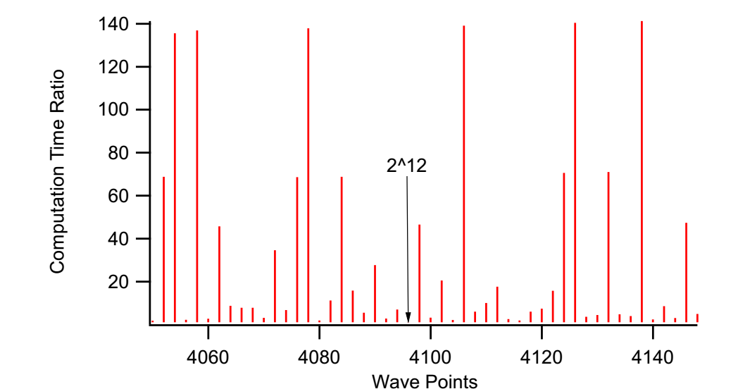
The arrow is at 4096 points (2^12). The moral of the story is that you should avoid wave sizes that have large prime factors. For example, a wave of 4078 takes a relatively long time - it has prime factors 2039 and 2. If you increase the size of the wave by two points, the computation is ~71 times faster (the prime factors of 4080 are 22223517). For best performance, the number of points should be a power of 2, e.g., 4096.

FFT Demos

Open FFT Swapping Demo

Open PSD Demo

Finding Magnitude and Phase

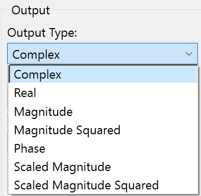
The FFT operation can create a complex, real, magnitude, magnitude squared, or phase result directly when you choose the desired Output Type:

If you choose to use the complex wave result of the FFT operation you can compute the magnitude and phase using WaveTransform (with keywords magnitude, magsqr, and phase), or with various procedures from the WaveMetrics Procedures folder (described in the next section).

If you want to unwrap the phase wave (to eliminate the phase jumps that occur between ±180 degrees), use the Unwrap operation or the Unwrap Waves dialog in the Data menu. See Unwrap. In two dimensions you can use the ImageUnwrapPhase operation.

Magnitude and Phase Using WaveMetrics Procedures

For backward compatibility you can compute FFT magnitude and phase using the WaveMetrics-provided procedures in the "WaveMetrics Procedures:Analysis:DSP (Fourier Etc)" folder.

You can access them using Igor's "#include" mechanism. See The Include Statement for instructions on including a procedure file.

The WM Procedures Index help file, which you can access from the Help→Help Windows menu, is a good way to find out what routines are available and how to access them.

FTMagPhase Functions

The FTMagPhase functions provide an easy interface to Igor's FFT operation. FTMagPhase has the following features:

Automatic display of the results.
Original data is untouched.
Can display magnitude in decibels.
Optional phase display in degrees or radians.
Optional 1D phase unwrapping.
Resolution enhancement.
Supports non-power-of-two data with optional windowing.

Use #include <FTMagPhase> in your procedure file to access these functions.

FTMagPhaseThreshold Functions

The FTMagPhaseThreshold functions are the same as the FTMagPhase procedures, but with an additional feature:

Phase values for low-amplitude signals may be ignored.

Use #include <FTMagPhaseThreshold> in your procedure file to access these functions.

DFTMagPhase Functions

The DFTMagPhase functions are similar to the FTMagPhase procedures, except that the slower Discrete Fourier Transform is used to perform the calculations:

User-selectable frequency start and end.
User-selectable number of frequency bands.

The procedures also include the DFTAtOneFrequency procedure, which computes the amplitude and phase at a single user-selectable frequency.

Use #include <DFTMagPhase> in your procedure file to access these functions.

CmplxToMagPhase Functions

The CmplxToMagPhase functions convert a complex wave, presumably the result of an FFT, into separate magnitude and phase waves. It has many of the features of FTMagPhase, but doesn't do the FFT.

Use #include <CmplxToMagPhase> in your procedure file to access these functions.

Spectral Windowing

The FFT computation makes an assumption that the input data repeats over and over. This is important if the initial value and final value of your data are not the same. A simple example of the consequences of this repeating data assumption follows.

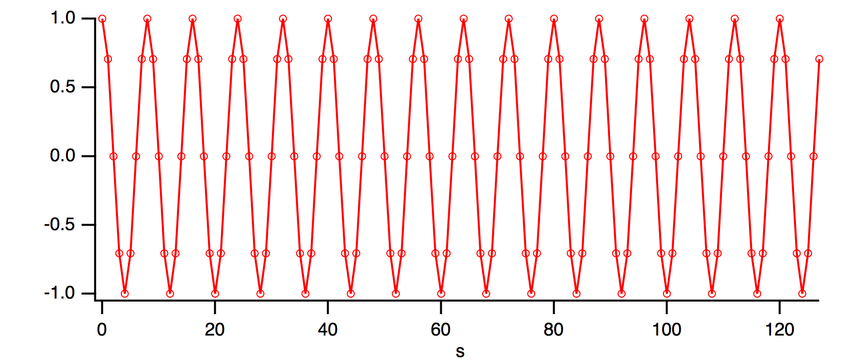
Suppose that your data is a sampled cosine wave containing 16 complete cycles:

Make/O/N=128 cosWave=cos(2*pi*p*16/128)
SetScale/P x 0, 1, "s", cosWave
Display cosWave
ModifyGraph mode=4,marker=8

Notice that if you copied the last several points of cosWave to the front, they would match up perfectly with the first several points of cosWave. In fact, let's do that with the Rotate operation:

Rotate 3,cosWave			// wrap last three values to front of wave
SetAxis bottom,-5,20		// look more closely there

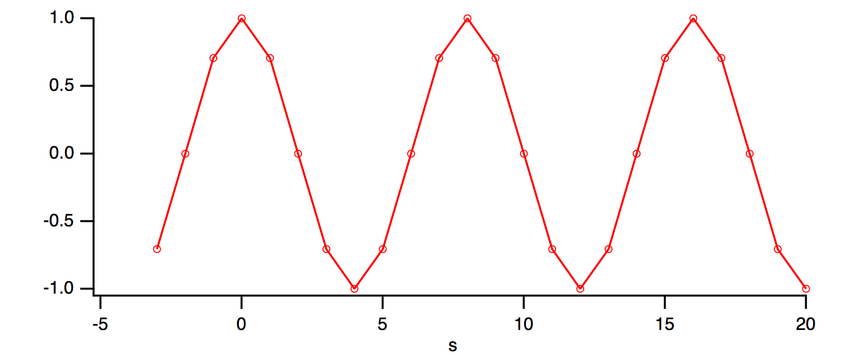
The rotated points appear at x=-3, -2, and -1. This indicates that there is no discontinuity as far as the FFT is concerned.

Because of the absence of discontinuity, the FFT magnitude result matches the ideal expectation:

Ideal FFT amplitude = cosine amplitude * number of points/2 = 1 * 128 / 2 = 64
FFT /OUT=3 /DEST=cosWaveF cosWave
Display cosWaveF
ModifyGraph mode=8, marker=8

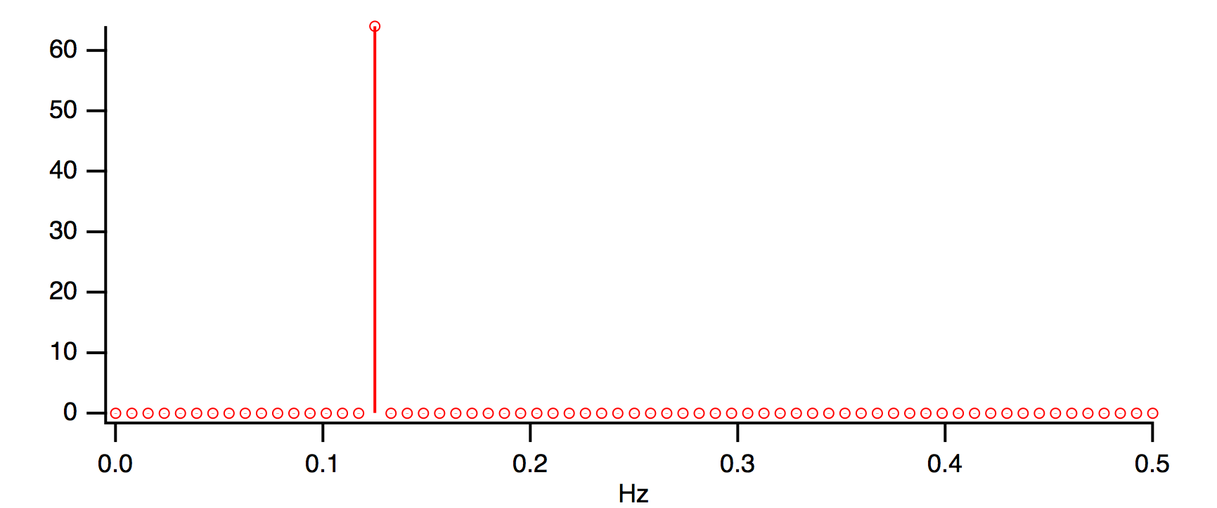
Notice that all other FFT magnitudes are zero. Now let us change the data so that there are 16.5 cosine cycles:

Make/O/N=128 cosWave = cos(2*pi*p*16.5/128)
SetScale/P x 0,1,"s", cosWave
SetAxis/A

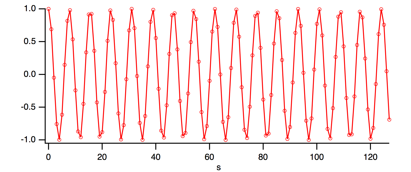
When we rotate this data as before, you can see what the FFT will perceive to be a discontinuity between the point 127 and point 0 of the unrotated data. In this next graph, the original point 127 has been rotated to x= -1 and point 0 is still at x=0.

Rotate 3, cosWave
SetAxis bottom, -5, 20

When the FFT of this data is computed, the discontinuity causes "leakage" of the main cosine peak into surrounding magnitude values.

FFT /OUT=3 /DEST=cosWaveF cosWave
SetAxis/A

How does all this relate to spectral windowing? Spectral windowing reduces this leakage and gives more accurate FFT results. Specifically, windowing reduces the number of adjacent FFT values affected by leakage. A typical window accomplishes this by smoothly attenuating both ends of the data towards zero.

Hanning Window

Windowing the data before the FFT is computed can reduce the leakage demonstrated above. The Hanning window is a simple raised cosine function defined by the equation:

{hanning}[p]=\frac{1-\cos \left(\displaystyle \frac{2 \pi p}{N-1}\right)}{2}

Let us apply the Hanning window to the 16.5 cycle cosine wave data:

Make/O/N=128 cosWave=cos(2*pi*p*16.5/128)
Hanning cosWave
Display cosWaveH
ModifyGraph mode=4, marker=8

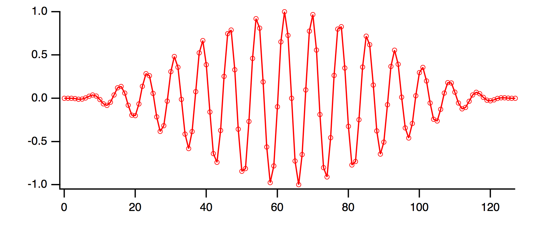
By smoothing the ends of the wave to zero, there is no discontinuity when wrapping around the ends.

In applying a window to the data, energy is lost. Depending on your application you may want to scale the output to account for coherent or incoherent gain. The coherent gain is sometimes expressed in terms of amplitude factor and it is equal to the sum of the coefficients of the window function over the interval. The incoherent gain is a power factor defined as the sum of the squares of the same coefficients. In the case that we are considering the correction factor is just the reciprocal of the coherent gain of the Hanning window

\displaystyle \text { coherent gain } \equiv \int_{0}^{1} \frac{1-\cos (2 \pi x / N)}{2} d x=0.5

so we can multiply the FFT amplitudes by 2 to correct for them:

cosWave *= 2							// Account for coherent gain
FFT /OUT=3 /DEST=cosWaveH cosWave
Display cosWaveH
ModifyGraph mode=4, marker=8

Note that frequency values in the neighborhood of the peak are less affected by the leakage, and that the amplitude is closer to the ideal of 64.

Other Windows

The Hanning window is not the ultimate window. Other windows that suppress more leakage tend to broaden the peaks. The FFT and WindowFunction operations have the following built-in windows: Hanning, Hamming, Bartlett, Blackman, Cosa(x), KaiserBessel, Parzen, Riemann, and Poisson.

You can create other windows by writing a user-defined function or by executing a simple wave assignment statement such as this one which applies a triangle window:

data *= 1-abs(2*p/numpnts(data)-1)

Use point indexing to avoid X scaling complications. You can determine the effect a window has by applying it to a perfect cosine wave, preferably a cosine wave at 1/4 of the sampling frequency (half the Nyquist frequency).

Other windows are provided in the WaveMetrics-supplied "DSP Window Functions" procedure file.

Multidimensional Windowing

When performing FFTs on images, artifacts are often produced because of the sharp boundaries of the image. As is the case for 1D waves, windowing of the image can help yield better results from the FFT.

To window images, you will need to use the ImageWindow operation, which implements the Hanning, Hamming, Bartlett, Blackman, and Kaiser windowing filters. See the ImageWindow operation for further details. For a windowing example, see Correlation or the Image Processing tutorial.

Power Spectra

Periodogram

The periodogram of a signal s(t) is an estimate of the power spectrum given by

\displaystyle P(f)=\frac{|F(f)|^{2}}{N},

where F(f) is the Fourier transform of s(t) computed by a Discrete Fourier Transform (DFT) and N is the normalization (usually the number of data points).

You can compute the periodogram using the FFT but it is easier to use the DSPPeriodogram operation, which has the same built-in window functions but you can also select your own normalization to suppress the DC term or to have the results expressed in dB as:

20log10(F/F0)

10log10(P/P0)

where P0 is either the maximum value of P or a user-specified reference value.

DSPPeriodogram can also compute the cross-power spectrum, which is the product of the Fourier transform of the first signal with the complex conjugate of the Fourier transform of the second signal:

\displaystyle P(f)=\frac{F(f) G^{*}(f)}{N},

where F(f) and G(f) are the DFTs of the two waves.

Power Spectral Density Functions

The PowerSpectralDensity routine supplied in the "Power Spectral Density" procedure file computes Power Spectral Density by averaging power spectra of segments of the input data. This is an early procedure file that does not take advantage of the new built-in features of the FFT or DSPPeriodogram operations. The procedure is still supported for backwards compatibility.

The PowerSpectralDensity functions take a long data wave on input and calculate the power spectral density function. These procedures have the following features:

Automatic display of the results.
Original data is untouched.
Pop-up list of windowing functions.
User setable segment length.

Use #include <Power Spectral Density> in your procedure file to access these functions. See The Include Statement for instructions on including a procedure file.

PSD Demo Experiment

The PSD Demo (in the Examples:Analysis: folder) uses the PowerSpectralDensity procedure and explains how it works in great detail, including justification for the scaling applied to the result.

Hilbert Transform

The Hilbert transform of a function f(x) is defined by

\displaystyle F_{H}(x)=\frac{1}{\pi} \int_{-\infty}^{\infty} \frac{f(t)}{t-x} d t.

The integral is evaluated as a Cauchy principal value. For numerical computation it is customary to express the integral as the convolution

\displaystyle F_{H}(x)=\left(\frac{-1}{\pi x}\right) \otimes f(x) .

Noting that the Fourier transform of (-1/πx) is i*sgn(x) we can evaluate the Hilbert transform using the convolution theorem of Fourier transforms. The HilbertTransform operation serves as a convenient shortcut. In the following example we compute the Hilbert transform of a cosine function which gives us a sine function:

Make/N=512 cosWave=cos(2*pi*x*20/512)
HilbertTransform/Dest=hCosWave cosWave
Display cosWave,hCosWave
ModifyGraph rgb(hCosWave)=(0,0,65535)

Time Frequency Analysis

When you compute the Fourier spectrum of a signal you dispose of all the phase information contained in the Fourier transform. You can find out which frequencies a signal contains but you do not know when these frequencies appear in the signal. For example, consider the signal

\displaystyle f(t)=\left\{\begin{array}{cc} \sin \left(2 \pi f_{1} t\right) & 0 \leq t<t_{1} \\ \\ \sin \left(2 \pi f_{2} t\right) & t_{1} \leq t<t_{2} \end{array} .\right.

The spectral representation of f(t) remains essentially unchanged if we interchange the two frequencies f₁ and f₂. In other words, the Fourier spectrum is not the best analysis tool for signals whose spectra fluctuate in time. One solution to this problem is the so-called "short time Fourier Transform", in which you can compute the Fourier spectra using a sliding temporal window. By adjusting the width of the window you can determine the time resolution of the resulting spectra.

Two additional tools for time-frequency analysis are the Wigner transform and the Continuous Wavelet Transform (CWT).

Wigner Transform

The Wigner transform (also known as the Wigner Distribution Function or WDF) maps a 1D time signal U(t) into a 2D time-frequency representation. Conceptually, the WDF is analogous to a musical score where the time axis is horizontal and the frequencies (notes) are plotted on a vertical axis. The WDF is defined by the equation

\displaystyle W(t, v)=\int_{-\infty}^{\infty} U(t+x / 2) U^{*}(t-x / 2) e^{-i 2 \pi x v} d x.

Note that the WDF W(t,ν) is real (this can be seen from the fact that it is a Fourier transform of an Hermitian quantity). The WDF is also a 2D Fourier transform of the Ambiguity function.

The localized spectrum can be derived from the WDF by integrating it over a finite area dtdn. Using Gaussian weight functions in both t and n, and choosing the minimum uncertainty condition dtdn=1, we obtain an estimate for the local spectrum

\displaystyle \widehat{W}(t, v ; \delta t) \propto\left|\int U\left(t^{\prime}\right) \exp \left[-2 \pi\left(\frac{t-t^{\prime}}{\delta t}\right)\right] \exp \left(-i 2 \pi v t^{\prime}\right) d t^{\prime}\right|^{2}.

To illustrate an application of the WignerTransform operation, consider the two-frequency signal:

Make/N=500 signal
signal[0,350]=sin(2*pi*x*50/500)
signal[250,]+=sin(2*pi*x*100/500)
WignerTransform /GAUS=100 signal
DSPPeriodogram signal				// Spectrum for comparison
Display signal

The signal used in this example consists of two "pure" frequencies that have small amount of temporal overlap:

Display; AppendImage M_Wigner

The temporal dependence is clearly seen in the Wigner transform. Note that the horizontal (time) transitions are not sharp. This is mostly due to the application of the minimum uncertainty relation dtdn=1 but it is also due to computational edge effects. By comparison, the spectrum of the signal while clearly showing the presence of two frequencies it provides no indication of the temporal variation of the signal's frequency content. Furthermore, the different power in the two frequencies may be attributed to either a different duration or a different amplitude.

Display W_Periodogram

Continuous Wavelet Transform

The Continuous Wavelet Transform (CWT) is a time-frequency representation of signals that graphically has a superficial similarity to the Wigner transform.

A wavelet transform is a convolution of a signal s(t) with a set of functions which are generated by translations and dilations of a main function. The main function is known as the mother wavelet and the translated or dilated functions are called wavelets. Mathematically, the CWT is given by

\displaystyle W(a, b)=\frac{1}{\sqrt{a}} \int s(t) \psi\left(\frac{t-b}{a}\right) d t .

Here b is the time translation and a is the dilation of the wavelet.

From a computational point of view it is natural to use the FFT to compute the convolution which suggests that the results are dependent on proper sampling of s(t).

When the mother wavelet is complex, the CWT is also a complex valued function. Otherwise the CWT is real. The squared magnitude of the CWT

\displaystyle |W(a, b)|^{2}

is equivalent to the power spectrum so that a typical display (image) of the CWT is a representation of the power spectrum as a function of time offset b. One should note however that the precise form of the CWT depends on the choice of mother wavelet y and therefore the extent of the equivalency between the squared magnitude of the CWT and the power spectrum is application dependent.

The CWT operation is implemented using both the FFT and the direct sum approach. You can use either one to get a representation of the effective wavelet using a delta function as an input. When comparing two CWT results you should always check that both use exactly the same definition of the wavelet function, same normalization and same computation method. For example,

Make/N=1000 signal=sin(2*pi*x*50/1000)
CWT/OUT=4/SMP2=1/R2={1,1,40}/WBI1=Morlet/WPR1=5/FSCL signal
Rename M_CWT, M_CWT1
Display as "Morlet FFT"; AppendImage M_CWT1

CWT/M=1/OUT=4/SMP2=1/R2={1,1,40}/WBI1=Morlet/FSCL /ENDM=2 signal
Rename M_CWT, M_CWT2
Display as "Morlet Direct Sum"; AppendImage M_CWT2

Using the complex Morlet wavelet in the direct sum method (/M=1) and displaying the squared magnitude we get:

CWT/M=1/OUT=4/SMP2=1/R2={1,1,40}/WBI1=MorletC/FSCL /ENDM=2 signal
Rename M_CWT, M_CWT3
Display as "Complex Morlet Direct Sum"; AppendImage M_CWT3

It is apparent that the last image has essentially the same results as the one generated using the FFT approach but in this case the edge effects are completely absent.

Discrete Wavelet Transform

The DWT is similar to the Fourier transform in that it is a decomposition of a signal in terms of a basis set of functions. In Fourier transforms the basis set consists of sines and cosines and the expansion has a single parameter. In wavelet transform the expansion has two parameters and the functions (wavelets) are generated from a single "mother" wavelet using dilation and offsets corresponding to the two parameters.

\displaystyle f(t)=\sum_{a} \sum_{b} c_{a b} \psi_{a b}(t),

where the two-parameter expansion coefficients are given by

\displaystyle c_{a b}=\int f(t) \psi_{a b}(t) d t

and the wavelets obey the condition

\displaystyle \psi_{a b}(t)=2^{a / 2} \Psi\left(2^{a} t-b\right) .

Here Y is the mother wavelet, a is the dilation parameter and b is the offset parameter.

The two parameter representation can complicate things quickly as one goes from 1D signal to higher dimensions. In addition, because the number of coefficients in each scale varies as a power of 2, the DWT of a 1D signal is not conveniently represented as a 2D image (as is the case with the CWT). It is therefore customary to "pack" the results of the transform so that they have the same dimensionality of the input. For example, if the input is a 1D wave of 128 (=27) points, there are 7-1=6 significant scales arranged as follows:

Scale	Storage Location
1	64-127
2	32-63
3	16-31
4	8-15
5	4-7
6	2-3

An interesting consequence of the definition of the DWT is that you can find out the shape of the wavelet by transforming a suitable form of a delta function. For example:

Make/N=1024 delta=0
delta[22]=1
DWT/I delta
Display W_DWT	// Daubechies 4 coefficient wavelet

Time Frequency Demos

Open CWT Demo.

Open Wigner Demo.

Convolution

You can use convolution to compute the response of a linear system to an input signal. The linear system is defined by its impulse response. The convolution of the input signal and the impulse response is the output signal response. Convolution is also the time-domain equivalent of filtering in the frequency domain.

Smoothing is also a form of convolution – see Smoothing.

The FilterFIR operation implements convolution in the time domain – see Digital Filtering.

Igor implements general convolution with the Convolve operation. To use the Convolve operation, choose Analysis→Convolve.

The built-in Convolve operation computes the convolution of two waves named "source" and "destination" and overwrites the destination wave with the results. The operation can also convolve a single source wave with multiple destination waves (overwriting the corresponding destination wave with the results in each case). The Convolve dialog allows for more flexibility by preduplicating the second waves into new destination waves.

If the source wave is real-valued, each destination wave must be real-valued and if source wave is complex, each destination wave must be complex, too. Double and single precision waves may be freely intermixed; the calculations are performed in the higher precision.

Convolve combines neighboring points before and after the point being convolved, so at the ends of the waves not enough neighboring points exist. The Convolve dialog presents three algorithms in the Algorithm group to deal with these missing points. Depending on the algorithm chosen, the destination waves' lengths may increase by the length of the source wave, less one.

The Linear algorithm is similar to the Smooth operation's Zero end effect method; zeros are substituted for the values of missing neighboring points.

The Circular algorithm is similar to the Wrap end effect method; this algorithm is appropriate for data which is assumed to endlessly repeat.

The acausal algorithm is a special case of Linear which eliminates the time delay that Linear introduces.

Depending on the algorithm chosen, the number of points in the destination waves may increase by the number of points in the source wave, less one. For linear and acausal convolution, the destination wave is first zero-padded by one less than the number of points in the source wave. This prevents the "wrap-around" effect that occurs in circular convolution. The zero-padded points are removed after acausal convolution, and retained after linear convolution.

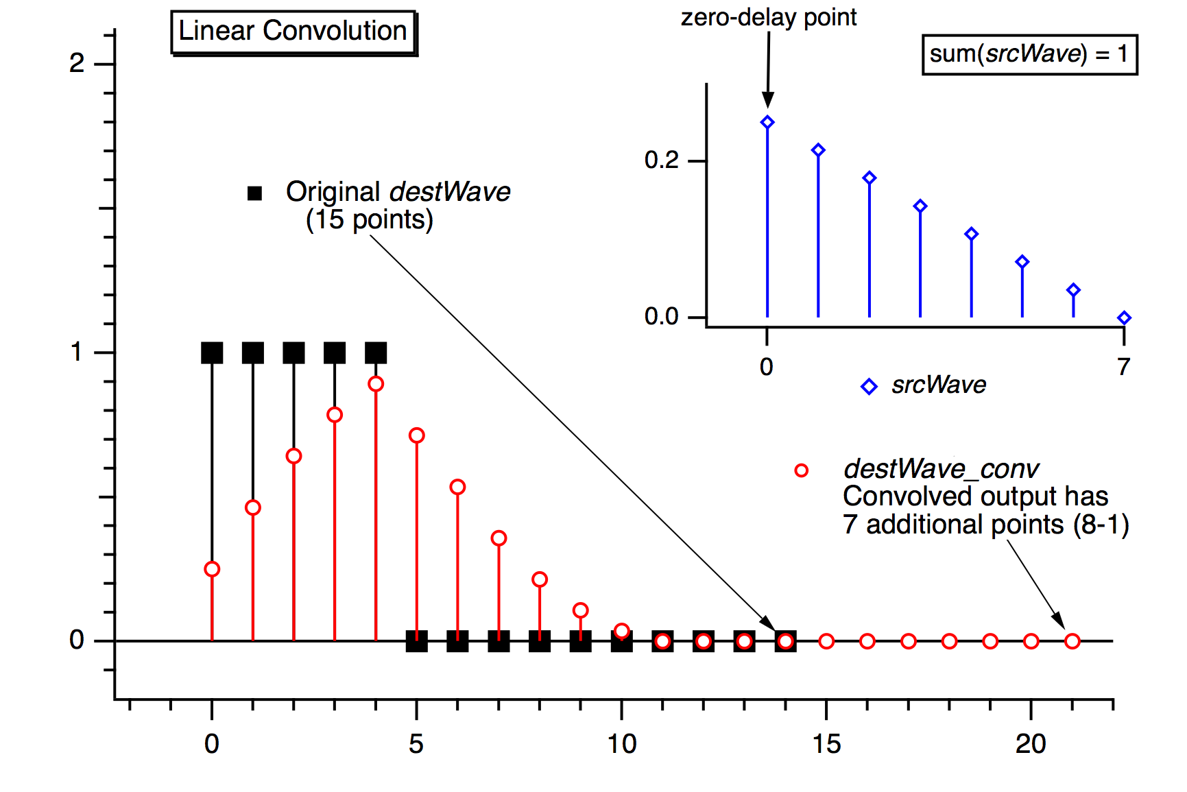
Use linear convolution when the source wave contains an impulse response (or filter coefficients) where the first point of srcWave corresponds to no delay (t = 0).

Use Circular convolution for the case where the data in the source wave and the destination waves are considered to endlessly repeat (or "wrap around" from the end back to the start), which means no zero padding is needed.

Use acausal convolution when the source wave contains an impulse response where the middle point of the source wave corresponds to no delay (t = 0).

Correlation

You can use correlation to compare the similarity of two sets of data. Correlation computes a measure of similarity of two input signals as they are shifted by one another. The correlation result reaches a maximum at the time when the two signals match best. If the two signals are identical, this maximum is reached at t = 0 (no delay). If the two signals have similar shapes but one is delayed in time and possibly has noise added to it then correlation is a good method to measure that delay.

Igor implements correlation with the Correlate operation. You can select Correlate from the Analysis menu. The source wave may also be a destination wave, in which case afterwards it will contain the "auto-correlation" of the wave. If the source and destination are different, this is called "cross-correlation".

The same considerations about combining differing types of source and destination waves applies to correlation as to convolution. Correlation must also deal with end effects, and these are dealt with by the circular and linear correlation algorithm selections. See Convolution.

Level Detection

Level detection is the process of locating the X coordinate at which your data passes through or reaches a given Y value. This is sometimes called "inverse interpolation". Stated another way, level detection answers the question: "given a Y level, what is the corresponding X value?" Igor provides two kinds of answers to that question.

One answer assumes your Y data is a list of unique Y values that increases or decreases monotonically. In this case there is only one X value that corresponds to a Y value. Since search position and direction don't matter, a binary search is most appropriate. For this kind of data, use the BinarySearch or BinarySearchInterp functions.

The other answer assumes that your Y data varies irregularly, as it would with acquired data. In this case, there may be multiple X values that cross the Y level; the X value returned depends on where the search starts and the search direction through the data. The FindLevel, FindLevels, EdgeStats, and PulseStats operations deal with this kind of data.

A related, but different question is "given a function y = f(x), find x where y is zero (or some other value)". This question is answered by the FindRoots operation. See Finding Function Roots and the FindRoots operation.

The following sections pertain to detecting level crossings in data that varies irregularly. The operations discussed are not designed to detect peaks; see Peak Measurement.

Finding a Level in Waveform Data

You can use the FindLevel operation to find a single level crossing, or the FindLevels operation to find multiple level crossings in waveform data. Both of these operations can optionally smooth the waves they search to reduce the effects of noise. A subrange of the data can be searched, by either ascending or descending X values, depending on the startX and endX values you supply to the operation's /R flag.

FindLevel locates the first level crossing encountered in the search range, starting at startX and proceeding toward endX until a level crossing is found. The search is performed sequentially. The outputs of FindLevel are two special numeric variables: V_Flag and V_LevelX. V_Flag indicates the success or failure of the search (0 is success), and V_LevelX contains the X coordinate of the level crossing.

For example, given the following data:

the command:

FindLevel/R=(-0.5,0.5) signal,0.30

prints this level crossing information into the history area:

V_Flag=0; V_LevelX=-0.37497; V_rising=1;

Finding a Level in XY Data

You can find a level crossing in XY data by searching the Y wave and then figuring out where in the X wave that X value can be found. This requires that the values in the X wave be sorted in ascending or descending order. To ensure this, the command:

Sort xWave,xWave,yWave

sorts the waves so that the values in xWave are ascending, and the XY correspondence is preserved.

The following procedure finds the X location where a Y level is crossed within an X range, and stores the result in the output variable V_LevelX:

Function FindLevelXY()
	String swy,swx	// strings contain the NAMES of waves
	Variable startX=-inf,endX=inf	// startX,endX correspond to VALUEs in wx,
					// not any X scaling
	Variable level
	// Put up a dialog to get info from user
	Prompt swy,"Y Wave",popup WaveList("*",";","")
	Prompt swx,"X Wave",popup WaveList("*",";","")
	Prompt startX, "starting X value"
	Prompt endX, "ending X value"
	Prompt level, "level to find"
	DoPrompt "Find Level XY", swy,swx,startX, endX, level
	
	WAVE wx = $swx
	WAVE wy = $swy
	
	// Here's where the interesting stuff begins
	Variable startP,endP	// compute point range covering startX,endX
	startP=BinarySearch(wx,startX)
	endP=BinarySearch(wx,endX)
	FindLevel/Q/R=[startP,endP] wy,level	// search Y wave, assume success
	Variable p1,m
	p1=x2pnt(wy,V_LevelX-deltaX(wy)/2)	// x2pnt rounds; circumvent it
	// Linearly interpolate between two points in wx that bracket V_levelX in wy
	m=(V_LevelX-pnt2x(wy,p1))/(pnt2x(wy,p1+1)-pnt2x(wy,p1))		// slope
	V_LevelX=wx[p1] + m * (wx[p1+1] -wx[p1] )	// point-slope equation
End

This function does not handle a level crossing that isn't found; all that is missing is a test of V_Flag after searching the Y wave with FindLevel.

Edge Statistics

The EdgeStats operation produces simple statistics (measurements, really) on a region of a wave that is expected to contain a single edge as shown below. If more than one edge exists, EdgeStats works on the first edge it finds. The edge statistics are stored in special variables which are described in the EdgeStats reference. The statistics are edge levels, X or point positions of various found "points", and the distances between them. These found points are actually the locations of level crossings, and are usually located between actual waveform points (they are interpolation locations).

EdgeStats is based on the same principles as FindLevel. EdgeStats does not work on an XY pair. See Converting XY Data to a Waveform.

Pulse Statistics

The PulseStats operation produces simple statistics (measurements) on a region of a wave that is expected to contain three edges as shown below. If more than three edges exist, PulseStats works on the first three edges it finds. PulseStats handles two other cases in which there are only one or two edges. The pulse statistics are stored in special variables which are described in the PulseStats reference.

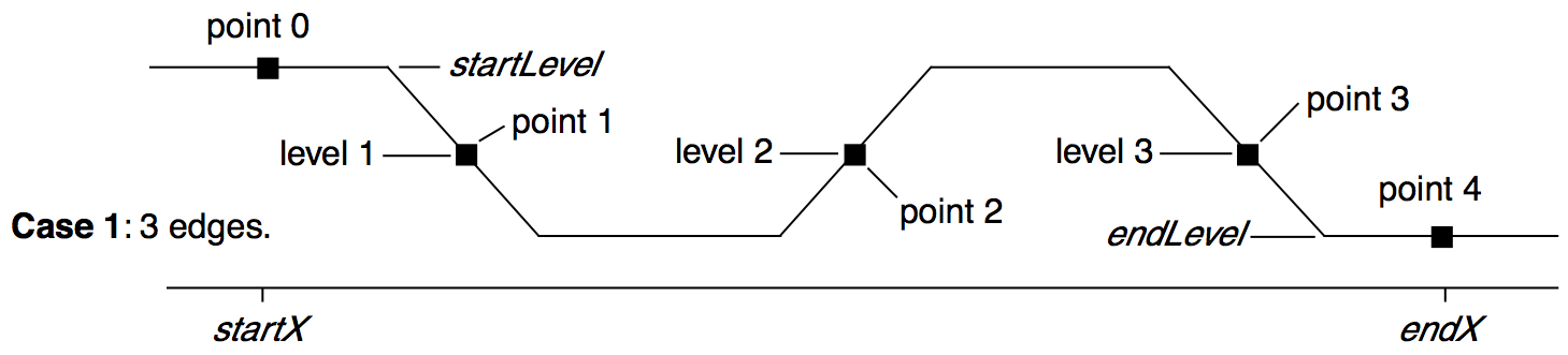
PulseStats is based on the same principles as EdgeStats. PulseStats does not work on an XY pair. See Converting XY Data to a Waveform.

Peak Measurement

The building block for peak measurement is the FindPeak operation. You can use it to build your own peak measurement procedures or you can use procedures provided by WaveMetrics.

Our Multipeak Fitting package provides a powerful GUI and programming interface for curve fitting to peak data. It can fit a number of peak shapes and baseline functions. A demo experiment provides an introduction: Open Multipeak Fitting Demo Experiment

We have created several peak finding and peak fitting Technical Notes. They are described in a summary Igor Technical Note, TN020s-Choosing a Right One.ifn in the Technical Notes folder. There is also an example experiment, called Multi-peak Fit, that does fitting to multiple Gaussian, Lorentzian and Voigt peaks. Multi-peak Fit is less comprehensive but easier to use than Tech Note 20.

The FindPeak operation searches a wave for a minimum or maximum by analyzing the smoothed first and second derivatives of the wave. The smoothing and differentiation is done on a copy of the input wave (so that the input wave is not modified). The peak maximum is detected at the smoothed first derivative zero-crossing, where the smoothed second derivative is negative. The position of the minimum or maximum is returned in the special variable V_PeakLoc. This and other special variables set by FindPeak are described in the operation reference.

The following describes the process that FindPeak goes through when it executes a command like this:

FindPeak/M=0.5/B=5 peakData		// 5 point smoothing, min level = 0.5

The box smoothing is performed first:

Then two central-difference differentiations are performed to find the first and second derivatives:

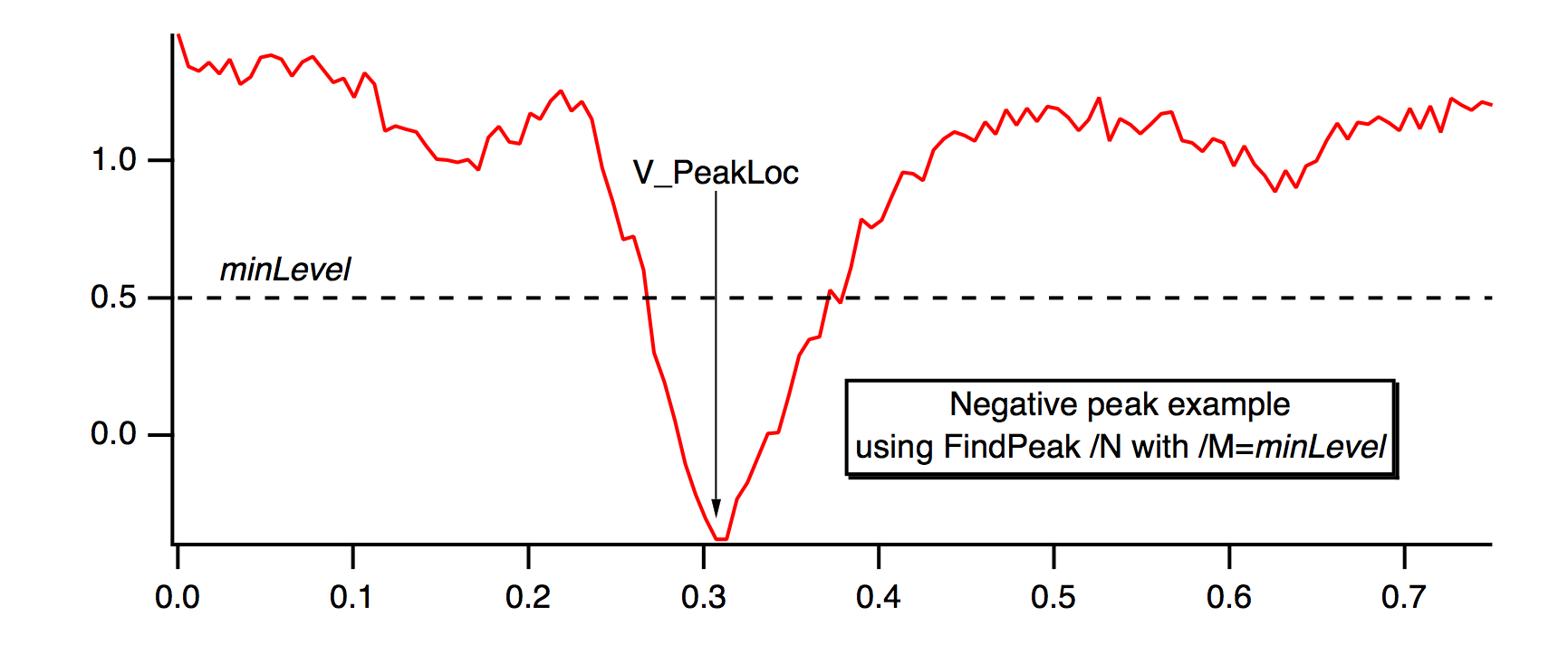
If you use the /M=minLevel flag, FindPeak ignores peaks that are lower than minLevel (i.e., the Y value of a found peak must exceed minLevel). The minLevel value is compared to the smoothed data, so peaks that appear to be large enough in the raw data may not be found if they are very near minLevel. If /N is also specified (search for minimum or "negative peak"), FindPeak ignores peaks whose amplitude is greater than minLevel (i.e., the Y value of a found peak will be less than minLevel). For negative peaks, the peak minimum is at the smoothed first derivative zero-crossing, where the smoothed second derivative is positive.

This command shows an example of finding a negative peak:

FindPeak/N/M=0.5/B=5 negPeakData		// 5 point smoothing, max level=0.5

To find multiple peaks, write a procedure that calls FindPeak from within a loop. After a peak is found, restrict the range of the search with /R so that the just-found peak is excluded, and search again. Exit the loop when V_Flag indicates a peak wasn't found.

The FindPeak operation does not work on an XY pair. See Converting XY Data to a Waveform.

Smoothing

Smoothing is a specialized filtering operation used to reduce the variability of data. It is sometimes used to reduce noise.

This section discusses smoothing 1-dimensional waveform data with the Smooth, FilterFIR, and Loess operations. Also see the FIlterIIR and Resample operations.

note

Smoothing XY data can be handled by the Loess operation and the Median.ipf procedure file (see Median Smoothing).

note

Smoothing image and 3D data is handled by the MatrixFilter, MatrixConvolve, and ImageFilter operations.

Igor has several built-in 1D smoothing algorithms. In addition, you can supply your own smoothing coefficients.

Choose Smooth from the Analysis menu. Depending on the smoothing algorithm chosen, there may be additional parameters to specify in the dialog.

Built-in Smoothing Algorithms

Igor has numerous built-in smoothing algorithms for 1-dimensional waveforms, and one that works with The XY Model of Data:

Algorithm	Operation	Data
Binomial	Smooth	1D waveform
Savitzky-Golay	Smooth/S	1D waveform
Box (Average)	Smooth/B	1D waveform
Custom Smoothing	FilterFIR	1D waveform
Median	Smooth/M	1D waveform
Percentile, Min, Max	Smooth/M/MPCT	1D waveform
Loess	Loess	1D waveform, XY 1D waves, false-color images, matrix surfaces, and multivariate data*.

* The Loess operation supports these data formats, but the Smooth dialog does not provide an interface to select them.

The first four algorithms precompute or apply one set of smoothing coefficients according to the smoothing parameters, and then replaces each data wave with the convolution of the wave with the coefficients.

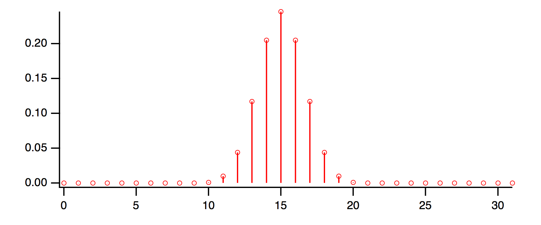
You can determine what coefficients have been computed by smoothing a wave containing an impulse. For instance:

Make/O/N=32 wave0=0; wave0[15]=1; Smooth 5,wave0   // Smooth an impulse
Display wave0; ModifyGraph mode=8,marker=8         // Observe coefficients

Compute the FFT of the coefficients with magnitude output to view the frequency response. See Finding Magnitude and Phase.

The last two algorithms (the Smooth/M and Loess operations) are not based on creating a fixed set of smoothing coefficients and convolution, so this technique is not applicable.

Binomial Smoothing

The Binomial smoothing operation is a Gaussian filter. It convolves your data with normalized coefficients derived from Pascal's triangle at a level equal to the Smoothing parameter. The algorithm is derived from an article by Marchand and Marmet (1983).

This graph shows the frequency response of the binomial smoothing algorithm expressed as a percentage of the sampling frequency. For example, if your data is sampled at 1000 Hz and you use 5 passes, the signal at 200 Hz (20% of the sampling frequency) will be approximately 0.1.

Savitzky-Golay Smoothing

Savitzky-Golay smoothing uses a different set of precomputed coefficients popular in the field of chemistry. It is a type of Least Squares Polynomial smoothing. The amount of smoothing is controlled by two parameters: the polynomial order and the number of points used to compute each smoothed output value. This algorithm was first proposed by A. Savitzky and M.J.E. Golay in 1964. The coefficients were subsequently corrected by others in 1972 and 1978; Igor uses the corrected coefficients.

The maximum Points value is 32767; the minimum is either 5 (2nd order) or 7 (4th order). Note that 2nd and 3rd order coefficients are the same, so we list only the 2nd order choice. Similarly, 4th and 5th order coefficients are identical.

Even though Savitzky-Golay smoothing has been widely used, there are advantages to the binomial smoothing as described by Marchand and Marmet in their article.

The following graphs show the frequency response of the Savitzky-Golay algorithm for 2nd order and 4th order smoothing. The large responses in the higher frequencies show why binomial smoothing is often a better choice.

Box Smoothing

Box smoothing is similar to a moving average, except that an equal number of points before and after the smoothed value are averaged together with the smoothed value. The Points parameter is the total number of values averaged together. It must be an odd value, since it includes the points before, the center point, and the points after. For instance, a value of 5 averages two points before and after the center point, and the center point itself:

Make/O/N=32 wave0=0; wave0[15]=1; Smooth/B 5,wave0    // Smooth impulse
Display wave0; ModifyGraph mode=8,marker=8            // Observe coefficients

The following graph shows the frequency response of the box smoothing algorithm.

Median Smoothing

Median smoothing does not use convolution with a set of coefficients. Instead, for each point it computes the median of the values over the specified range of neighboring values centered about the point. NaN values in the waveform data are allowed and are excluded from the median calculations.

For simple XY data median smoothing, include the Median.ipf procedure file:

#include <Median>

and use the Analysis→Packages→Median XY Smoothing menu item. Currently this procedure file does not handle NaNs in the data and only implements method 1 as described below.

For image (2D matrix) median smoothing, use the MatrixFilter or ImageFilter operation with the median method. ImageFilter can smooth 3D matrix data.

There are several ways to use median smoothing (Smooth/M) on 1D waveform data:

Replace all values with the median of neighboring values.
Replace each value with the median if the value itself is NaN. See Replace Missing Data using Median Smoothing.
Replace each value with the median if the value differs from the median by a the specified threshold amount.
Instead of replacing the value with the computed median, replace it with a specified number, including 0, NaN, +inf, or -inf.

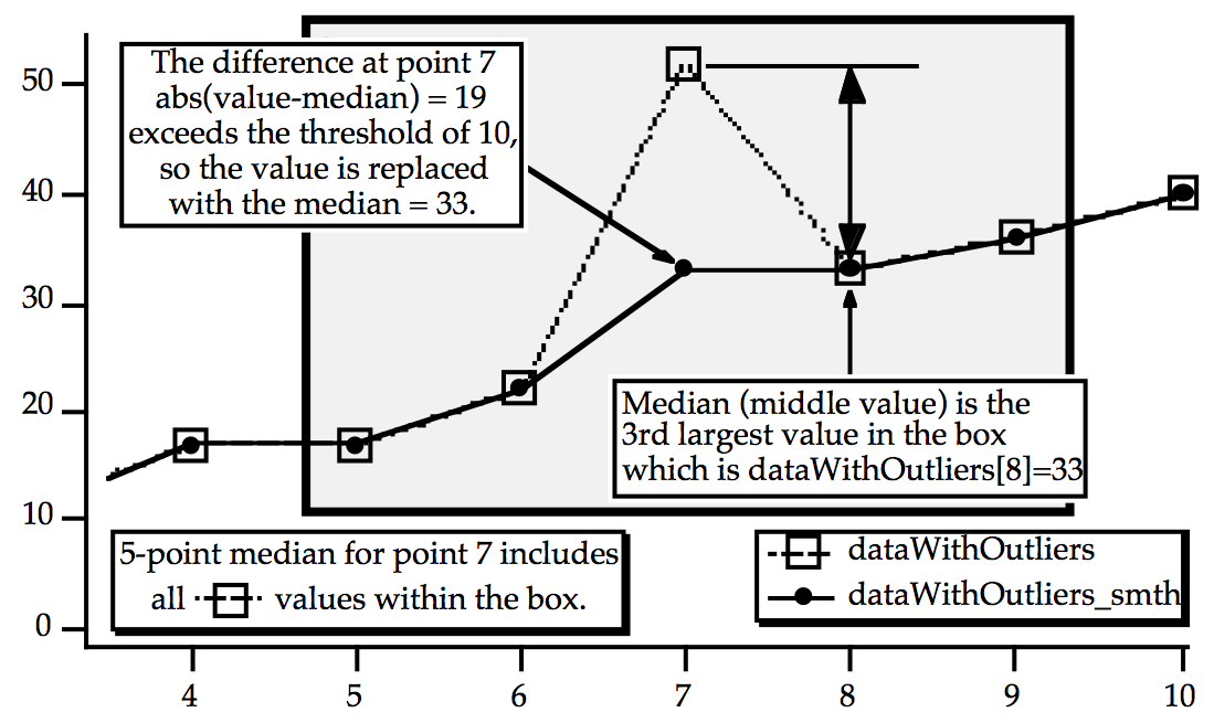
Median smoothing can be used to replace "outliers" in data. Outliers are data that seem "out of line" from the other data. One measure of this "out of line" is excessive deviation from the median of neighboring values. The Threshold parameter defines what is considered "excessive deviation".

// Example uses integer wave to simplify checking the results
Make/O/N=20/I dataWithOutliers= 4*p+gnoise(1.5) // simple line with noise
dataWithOutliers[7] *=2                         // make an outlier at point 7
Display dataWithOutliers
Duplicate/O dataWithOutliers,dataWithOutliers_smth
Smooth/M=10 5, dataWithOutliers_smth            // threshold=10, 5 point median
AppendToGraph  dataWithOutliers_smth

Percentile, Min, and Max Smoothing

Median smoothing is actually a specialization of Percentile smoothing, as are Min and Max.

Percentile smoothing returns the smallest value in the smoothing window that is greater than the smallest percentile % of the values:


percentile= 0:	(min) The smoothed value is the minimum value in the smoothing window. 0 is the minimum value for percentile.
percentile= 50:	(median) The smoothed value is the median of the values in the smoothing window.
percentile= 100:	(max) The smoothed value is the maximum value in the smoothing window. 100 is the maximum value for percentile.

As an example, assume that percentile = 25, the number of points in the smoothing window is 7, and for one input point the values in the window after sorting are:

{0, 1, 8, 9, 10, 11, 30}

The 25th percentile is found by computing the rank R:

R = (percentile /100) * (num + 1)

In this example, R evaluates to 2 so the second item in the sorted list, 1 in this example, is the percentile value for the input point.

The percentile algorithm uses an interpolated rank to compute the value of percentiles other than 0 and 100. See the Smooth operation for details.

Loess Smoothing

The Loess operation smooths data using locally-weighted regression smoothing. This algorithm is sometimes classified as a "nonparametric regression" procedure [Cleveland].

The regression can be constant, linear, or quadratic. A robust option that ignores outliers is available. In addition, for small data sets Loess can generate confidence intervals.

See the Loess operation help for a discussion of the basic and robust algorithms, examples, and references.

This implementation works with waveforms, XY pairs of waves, false-color images, matrix surfaces, and multivariate data (one dependent data wave with multiple independent variable data waves). Loess discards NaN input values.

The Smooth Dialog, however, provides an interface for only waveforms and XY pairs of waves (see The XY Model of Data), and does not provide an interface for confidence intervals or other less common options.

Here's an example from the Loess operation help of interpolating (smoothing) an XY pair and creating an interpolated 1D waveform (Y vs X scaling).

// 3.  1-D Y vs X wave data interpolated to waveform (Y vs X scaling)
//     with 99% confidence interval outputs (cp and cm)
// NOx = f(EquivRatio)
// Y wave
Make/O/D NOx = {4.818, 2.849, 3.275, 4.691, 4.255, 5.064, 2.118, 4.602, 2.286, 0.97, 3.965, 5.344, 3.834, 1.99, 5.199, 5.283, 3.752, 0.537, 1.64, 5.055, 4.937, 1.561};

// X wave (Note that the X wave is not sorted)
Make/O/D EquivRatio = {0.831, 1.045, 1.021, 0.97, 0.825, 0.891, 0.71, 0.801,  1.074, 1.148, 1, 0.928, 0.767, 0.701, 0.807, 0.902, 0.997, 1.224, 1.089, 0.973, 0.98, 0.665};

// Graph the input data
Display NOx vs EquivRatio; ModifyGraph mode=3,marker=19

// Interpolate to dense waveform over X range
Make/O/D/N=100 fittedNOx
WaveStats/Q EquivRatio
SetScale/I x, V_Min, V_max, "", fittedNOx
Loess/CONF={0.99, cp, cm}/DEST=fittedNOx/DFCT/SMTH=(2/3) srcWave=NOx,factors={EquivRatio}

// Display the fit (smoothed results) and confidence intervals
AppendtoGraph fittedNOx, cp,cm
ModifyGraph rgb(fittedNOx)=(0,0,65535)
ModifyGraph mode(fittedNOx)=2,lsize(fittedNOx)=2
Legend

note

Loess is memory intensive, especially when generating confidence intervals. Read the Memory Details section of the Loess operation help if you use confidence intervals.

Custom Smoothing Coefficients

You can smooth data with your own set of smoothing coefficients by selecting the Custom Coefs algorithm. Use this option when you have low-pass filter (smoothing) coefficients created by another program or by the Igor Filter Design Laboratory (IFDL).

Choose the wave that contains your coefficients from the pop-up menu that appears. Igor will convolve these coefficients with the input wave using the FilterFIR operation. You should use FilterFIR when convolving a short wave with a much longer one. Use the Convolve operation when convolving two waves with similar number of points; it's faster.

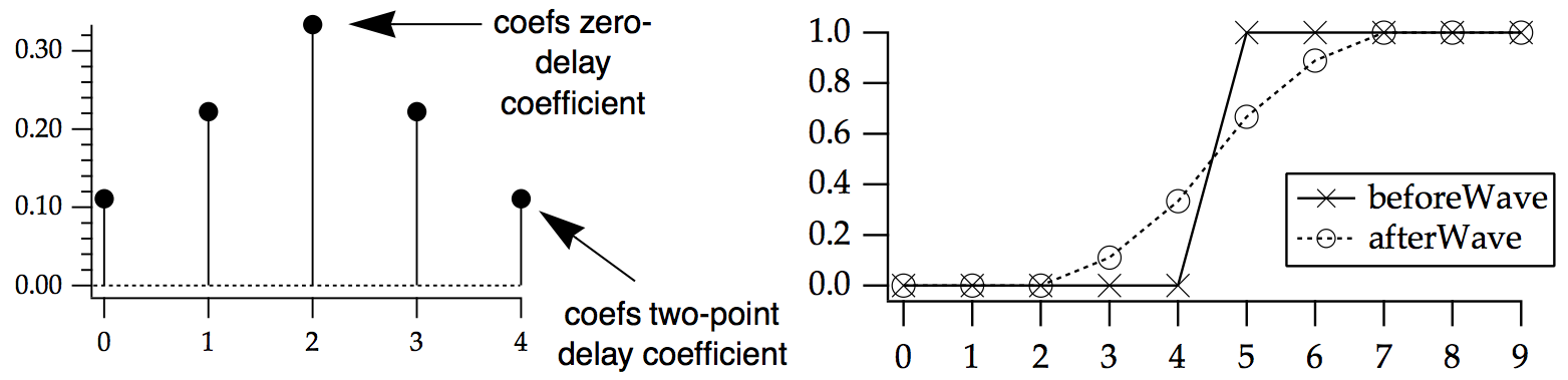
All the values in the coefficients wave are used. FilterFIR presumes that the middle point of the coefficient wave corresponds to the delay = 0 point. This is usually the case when the coefficient wave contains the two-sided impulse response of a filter, which has an odd number of points. (For a coefficient wave with an even number of points, the "middle" point is numpnts(coefs)/2-1, but this introduces a usually unwanted delay in the smoothed data).

In the following example, the coefs wave smooths the data by a simple 7 point Bartlett (triangle) window (omitting the first and last Bartlett window values which are 0):

// This example shows a unit step signal smoothed by a 7-point Bartlett window
Make/O/N=10 beforeWave = (p>=5)     // unit step at p == 5
Make/O coefs={1/3,2/3,1,2/3,1/3}    // 7 point Bartlett window
WaveStats/Q coefs
coefs/= V_Sum
Duplicate/O beforeWave,afterWave
FilterFIR/E=3/COEF=coefs afterWave
Display beforeWave,afterWave

End Effects

The first four smoothing algorithms compute the output value for a given point using the point's neighbors. Each algorithm combines an equal number of neighboring points before and after the point being smoothed. At the start or end of a wave some points will not have enough neighbors, so a method for fabricating neighbor values must be implemented.

You choose how Igor fabricates those values with the End Effect pop-up menu in the Smoothing dialog. In the descriptions that follow, i is a small positive integer, and wave[n] is the last value in the wave to be smoothed.

The Bounce method uses wave[i] in place of the missing wave[-i] values and wave[n-i] in place of the missing wave[n+i] values. This works best if the data is assumed to be symmetrical about both the start and the end of the wave. If you don't specify the end effect method, Bounce is used.

The Wrap method uses wave[n-i] in place of the missing wave[-i] values and vice-versa. This works best if the wave is assumed to endlessly repeat.

The Zero method uses 0 for any missing value. This works best if the wave starts and ends with zero.

The Repeat method uses wave[0] in place of the missing wave[-i] values and wave[n] in place of the missing wave[n+i] values. This works best for data representing a single event.

When in doubt, use Repeat.

Smoothing Demo

Open Smooth Curve Through Noise Demo

Digital Filtering

Digital filters are used to emphasize or de-emphasize frequencies present in waveforms. For example, low-pass filters preserve low frequencies and reject high frequencies.

Applying a filter to an input waveform results in a "response" output waveform.

Igor can design and apply Finite Impulse Response (FIR) and Infinite Impulse Response (IIR) digital filters.

Other forms of digital filtering exist in Igor, signficantly the various Smoothing operations, which includes Savitzky-Golay, Loess, median, and moving-average smoothing.

Using the Convolve operation directly is another way to perform digital filtering, but that requires more knowledge than using the Filter Design and Application Dialog discussed below.

The Igor Filter Design Laboratory (IFDL) package can also be used to design and apply digital filters.

Sampling Frequency and Design Frequency Bands

The XY Model of Data is not used in digital filtering. Use the Waveform Model of Data, and set the sampling frequency using SetScale or the Change Wave Scaling Dialog.

For example, a waveform sampled at 44.1KHz (the sample rate of music on a compact disc) should have its X scaling set by a command such as:

SetScale/P x, 0, 1/44100, "s", musicWave

Typically filters are designed by specifying frequency "bands" that define a range of frequencies and the desired response amplitude (gain) and phase in that band.

The range of frequencies that are possible range from 0 to one-half the sampling frequency of the signal, which is called the "Nyquist frequency". In the example of musicWave, the Nyquist frequency is 22,050 Hz, so filter designs for that waveform define frequency bands that end no higher than 22,050 Hz.

Filter Design Output

The result of a filter design is a set of filter "coefficients" that are used to implement the filtering. The coefficient values and format depend on the filter design type, number of bands, band frequencies, and other parameters that define the filter response. The formats for FIR and IIR designs are quite different.

FIR Filters

Finite Impulse Response (FIR) means that the filter's time-domain response to an impulse ("spike") is zero after a finite amount of time:

An FIR filter is a finite length, evenly-spaced time series of impulses with varying amplitudes that is convolved with an input signal to produce a filtered output signal.

The impulse response amplitudes are termed "weighting factors" or "coefficients". They are identical to the filter's response to a unit impulse. You can observe an FIR filter's frequency response by simply computing the FFT of the coefficients. If you set the X scaling of the coefficients to match the sampling frequency of the data it will be applied to, the FFT result's frequency range will be scaled to the data's Nyquist frequency. For default X scaling, the frequency range will be 0 to 0.5 Hz:

FIR filters are valued for their completely linear phase (constant delay for all frequencies), but they generally need many more coefficients than IIR filters do to achieve similar frequency responses. Consequently, electronic digital realizations of FIR filters are usually more expensive than the corresponding IIR filter.

You supply FIR coefficients to the FilterFIR operation along with the input waveform to compute the filtered output waveform.

IIR Filters

The response of an Infinite Impulse Response (IIR) filter continues indefinitely, as it does for analog electronic filters that employ inductors and capacitors:

An IIR filter is a set of coefficients or weights a0, a1, a2,… and b0, b1, b2… whose values and use depend on the digital implementation topology. Unlike the FIR filter, these coefficients are not the same as the filter's response to a unit impulse. See the IFDL IIR Filter Design topic for further explanation.

IIR filters can realize quite sophisticated frequency responses with very few coefficients. The drawbacks are non-linear phase, potential for numerical instability (oscillation) when realized using limited-precision arithmetic, and the indirect design methodology (frequency transformations of conventional analog filter methods).

Igor uses two IIR implementations:

Direct Form I (DF I)
Cascaded Bi-Quad Direct Form II (DF II)

The IIR coefficients are represented in three forms:

DF I
DF II
"zeros and poles" form (discussed in IFDL's IIR Analog Prototype Design Graph topic)

You supply IIR coefficients to the FilterIIR operation along with the input waveform to compute the filtered output waveform. The format of IIR design coefficients depends on the implementation, as you can see in tables showing coefficients for Direct Form 1, Cascaded Bi-Quad Direct Form II, and pole-zero implementations of the same filter design.

Filter Design and Application Dialog

The Filter Design and Application dialog provides a simple user-interface for designing and applying a digital filter. Choose Analysis→Filter to display it:

This dialog allows you to design a subset of the Igor Filter Design Laboratory (IFDL) filters. It is simpler and the filters are sufficient for most purposes.

Initially the Design FIR Filter tab is shown with a simple low-pass filter pre-selected. "Design using this Sampling Frequency (Hz)" is set to 1 and the frequencies shown are in the default range of 0 to 0.5 Hz because the default design sampling frequency is 1 Hz.

To start the filter design, either:

Manually enter the sampling frequency or
Click Apply Filter and select a wave to be filtered whose sampling frequency is properly set as described above

This fieldRecording wave was sampled at 48000 Hz:

Switch back to the Response tab to show the default low-pass filter using the entered sampling frequency. The frequency range is now 0-24000 Hz:

You can use any combination of one low-pass band, one high-pass band, and one notch to pass or reject frequency components of the sampled data wave. By using both low-pass and high-pass bands you can create Band-Pass and Band-Stop Filters.

Before we apply a filter to fieldRecording, let's graph the original waveform:

It is also helpful if you know the frequency content of the input wave before filtering. Use the Analysis→Transforms→Fourier dialog:

This signal has two interesting bands of frequencies: 0 to 4.5KHz and 4.5 to about 10KHz, as shown in the fieldRecording_FFT result:

For illustrative purposes, let's walk through designing two filters that isolate each band: a low-pass filter and a high-pass filter.

Example: Low-Pass FIR Filter

A low-pass filter can be designed to keep the signal frequencies below 4.5KHz and reject higher frequencies.

An infinitely sharp cutoff between those frequencies isn't practical – it takes an infinite number of coefficients – so we specify two frequencies over which the transition from pass band to reject band happens. The smaller this transition band is, the more coefficients are needed to get a useful rejection of the higher frequencies.

Let's choose a 200 Hz transition width (4400 to 4600 Hz) and look at the frequency response with a reasonable number of coefficients (the default of 101):

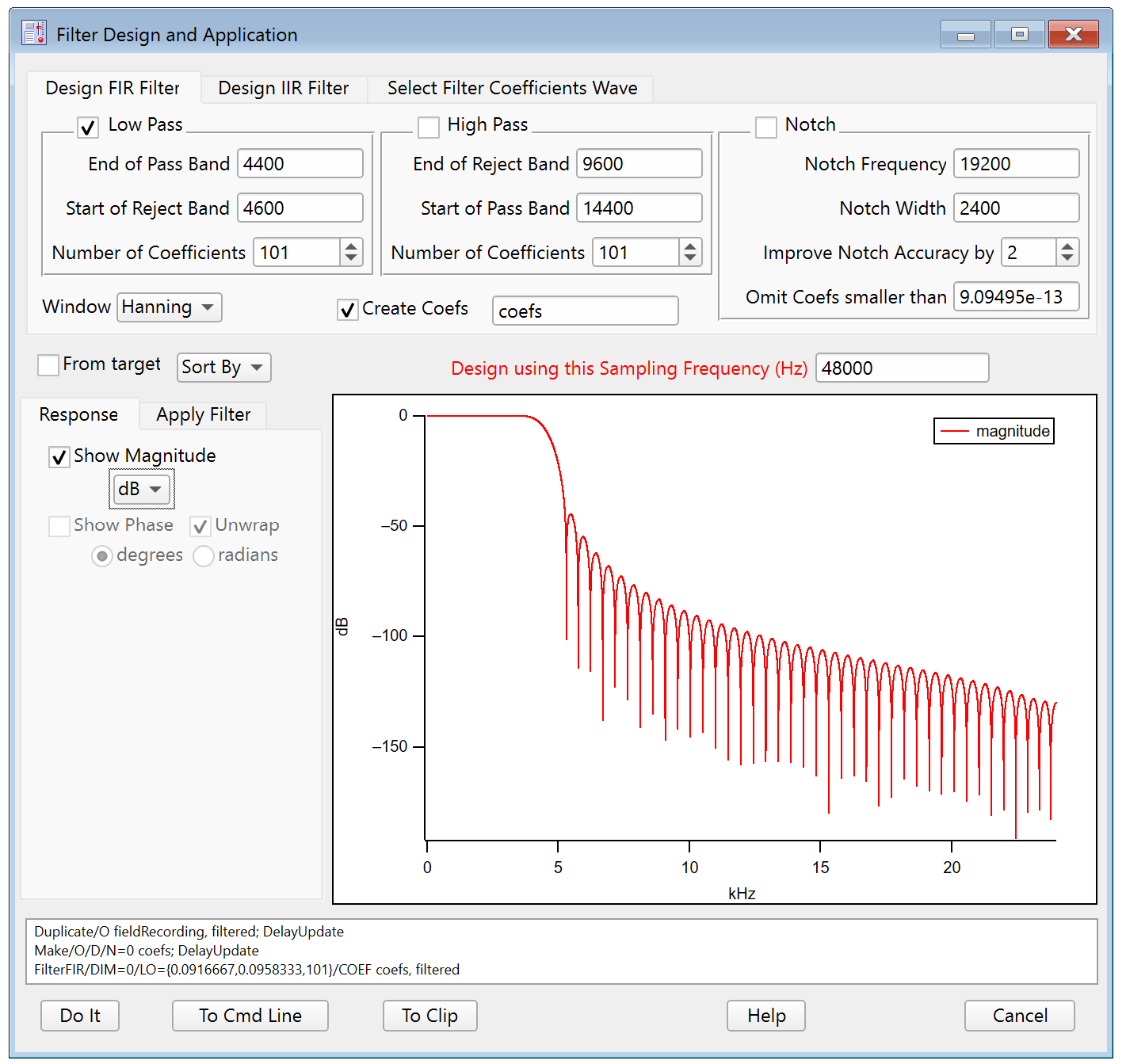
What does dB mean?

dB, an abbreviation for "decibel", is a logarithmic unit used to express the ratio of one value to another. In filtering it is the ratio of the output amplitude to the input amplitude at a given frequency. 0 dB means no change in ratio and is the ideal response of a filter in the pass band.

dB is computed as 20 * log(ratio) where ratio is output amplitude divided by input amplitude. So -100dB means a ratio of 10^-5 or 0.00001. You can see this by switching the response from dB to Gain and expanding the range vertically several times:

Choosing FIR Band Frequencies

You can avoid reducing the amplitude of frequencies near the end of the pass band by increasing the End of Pass Band frequency. A larger number of cofficients may be needed.

Choosing Number of Coefficients for FIR Designs

You can obtain a steeper transition from the pass band to the reject band by increasing the number of coefficients.

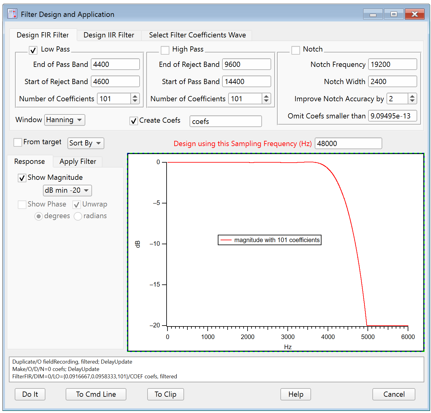
For an FIR filter, use an odd number of coefficients so that the the filtered output waveform is not delayed by a one-half sample.

Applying an FIR Filter to Data

Click the Apply Filter tab to see the result of applying the designed filter to a waveform.

Select the input wave in the Input to Filter listbox and click either Auto-update Filtered Output checkbox or the Update Output Now button. This updates a preview of the filtered result:

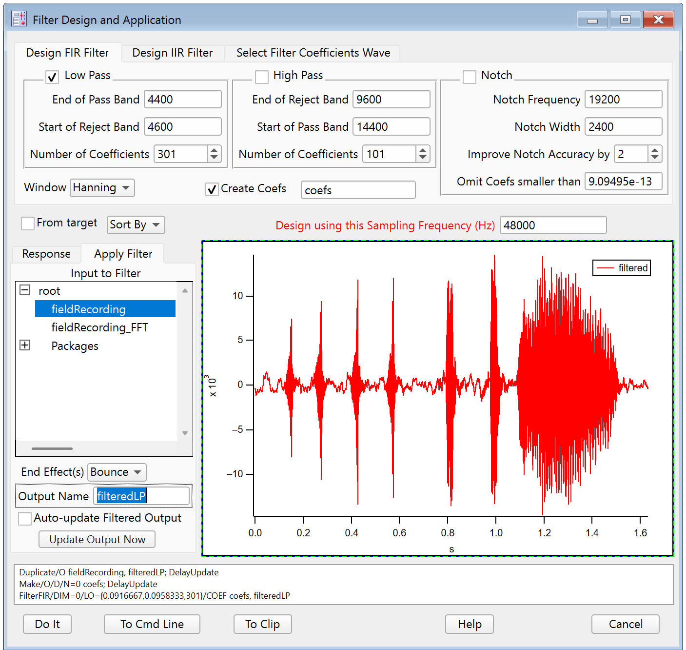
Click Do It to create a final output wave in the current data folder. You can set the name of the final output wave in the Output Name field. Here we used "filteredLP".

For comparision, here is the unfiltered fieldRecording:

The preview in the dialog shows that the higher-frequency elements are removed in the filtered output. An FFT of the filteredLP result verifies the change:

Applying an FIR Filter to Other Data

You can reuse a filter if you keep a copy of the design's output coefficients. For example:

Duplicate/O coefs, savedFIRfilter 		// Keep a copy of the filter design

You can apply the saved FIR filter to other data using the FilterFIR operation directly or using the Select Filter Coefficients Wave tab of the Filter dialog. Using the FilterFIR operation:

Duplicate/O otherData, otherDataFiltered
FilterFIR /DIM=0 /COEF=savedFIRfilter otherDataFiltered

Select Filter Coefficients Wave

This section shows how to apply a saved FIR or IIR filter to other data using the Filter Design and Application Dialog dialog.

First, Select the saved filter design wave in the Select Filter Coefficients Wave tab of the dialog.

You can view the filter's response by selecting the Response tab:

Second, select the wave to be filtered from the Apply Filter tab below:

Example: high-pass FIR Filter

Next we design a high-pass filter that preserves only the signal components that were removed by the low-pass filter.

Choose Analysis→Filter and set "Design using this Sampling Frequency (Hz)" to 48000.

Uncheck low-pass, check high-pass, and leave uncheck Notch.

Choosing high-pass FIR Band Frequencies

Set the End of Reject Band to 4400 and set Start of Pass Band to 4600 to define the same transition band as the low-pass filter that we created above. Use 301 terms to get a steep transition between rejecting low frequencies and passing high frequencies:

Click the Apply Filter tab to see the result of applying the designed filter to a waveform. Select the fieldRecording wave and click Update Output Now:

For comparision, here is the unfiltered fieldRecording:

The preview in the dialog shows that the lower-frequency elements are removed in the filtered output.

Click Do It to create the filteredHP result of high-pass filtering the fieldRecording waveform.

An FFT of the filteredHP result verifies the change:

Another way to evaluate the filtering result is to use the PlaySound operation on the original and filtered waveforms:

PlaySound fieldRecording
PlaySound filteredLP
PlaySound filteredHP

Example: Notch FIR Filter

A notch filter is usually employed to reject a very narrow range of frequencies that interfere with the desired signal. Removing the interference of 50 or 60 Hz power signals from phsyiological waveforms is one such use case.

Here is a synthesized waveform with a 5000 Hz sampling frequency, a 200 Hz signal, and 60 Hz interference. The graph on the right shows it's spectral content:

Check the Notch checkbox and uncheck the low-pass and high-pass checkboxes to create a notch-only filter.

The FilterFIR operation uses high-precision calculations to get a deep notch at the selected frequency, preferring to adjust the frequency to get deeper notches. The Improve Notch Accuracy value (nMult in the FilterFIR documentation) indirectly sets the number of coefficients used to implement the notch.

Here is the result of applying this filter design:

The interfering 60 Hz signal has been greatly diminished.

Other FIR Designs using IFDL

The FIR filters created using the Filter Design and Application dialog are simple filters created by applying a "window" shape - such as the Hanning WindowFunction - to truncated sin(x)/x kernels.

The filters are functional but require a lot of coefficients to get high performance (steep filter transition bands, good rejection of unwanted frequencies). Often these aren't important shortcomings, but if the designed filter is intended for actual electronic implementation, those extra coefficients get expensive.

High-performance FIR filters using far fewer coefficients can be computed by using the Igor Filter Design Laboratory (IFDL) package. It optimizes both filter response and the number of filter coefficients using the Remez Exchange algorithm as described in the seminal paper by McClellan, Parks, and Rabiner. See the Remez operation for additional references.

IIR Designs

The IIR filters created using the Filter Design and Application dialog are based on tranforms of analog Butterworth filters, a standard smooth-response filter of the electrical and mechanical engineering worlds. See IIR Filters for details.

Use the Igor Filter Design Laboratory (IFDL) to design IIR filters based on transforms of analog Bessel and Chebyshev filters.

Like the FIR Filters, the easily-designed IIR filters are specified in terms of filter type (low-pass, high-pass, notch) and design frequencies.

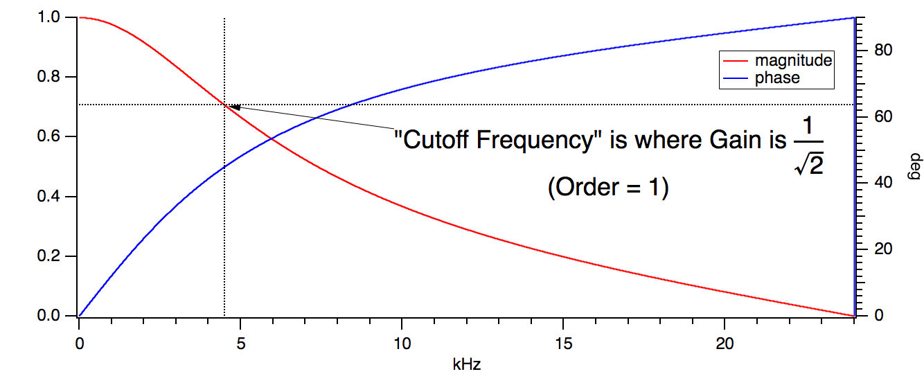
Choosing IIR Band Frequencies

Unlike FIR Design, the IIR Design uses a single cutoff frequency to define pass and reject bands. You can think of the cutoff frequency as the frequency where the response begins to "cut off" (reject) frequency components of the signal. "Begins" is chosen to be at the -3 dB point of the response, the so-called "half-power" amplitude, where the gain is 1/sqrt(2) = 0.707107:

Band-Pass and Band-Stop Filters

A filter that passes or rejects a range of frequencies that do not include 0 or the Nyquist frequency is called a band pass or band stop filter. Such filters are useful only for preserving or rejecting a narrow range of frequencies. A notch filter is a kind of band stop filter that has its own special implementation.

Band -Pass and Band- stop filters both use the low-pass and high-pass settings of the dialog. The difference is which cutoff frequency is lower than the other.

If the low-pass cutoff frequency is less than high-pass cutoff frequency, the result is a band stop filter:

If the high-pass cutoff frequency is less than low-pass cutoff frequency, the result is a band pass filter:

Choosing Order for IIR Designs

Instead of adjusting the number of coefficients to alter the performance of the filtering, IIR designs use a filter "order". Essentially, each order represents another layer of recursive filtering. A higher-order filter has steeper band transitions, more phase shift, and can be numerically less stable. Increasing the order from 1 to 6 creates a much steeper transition:

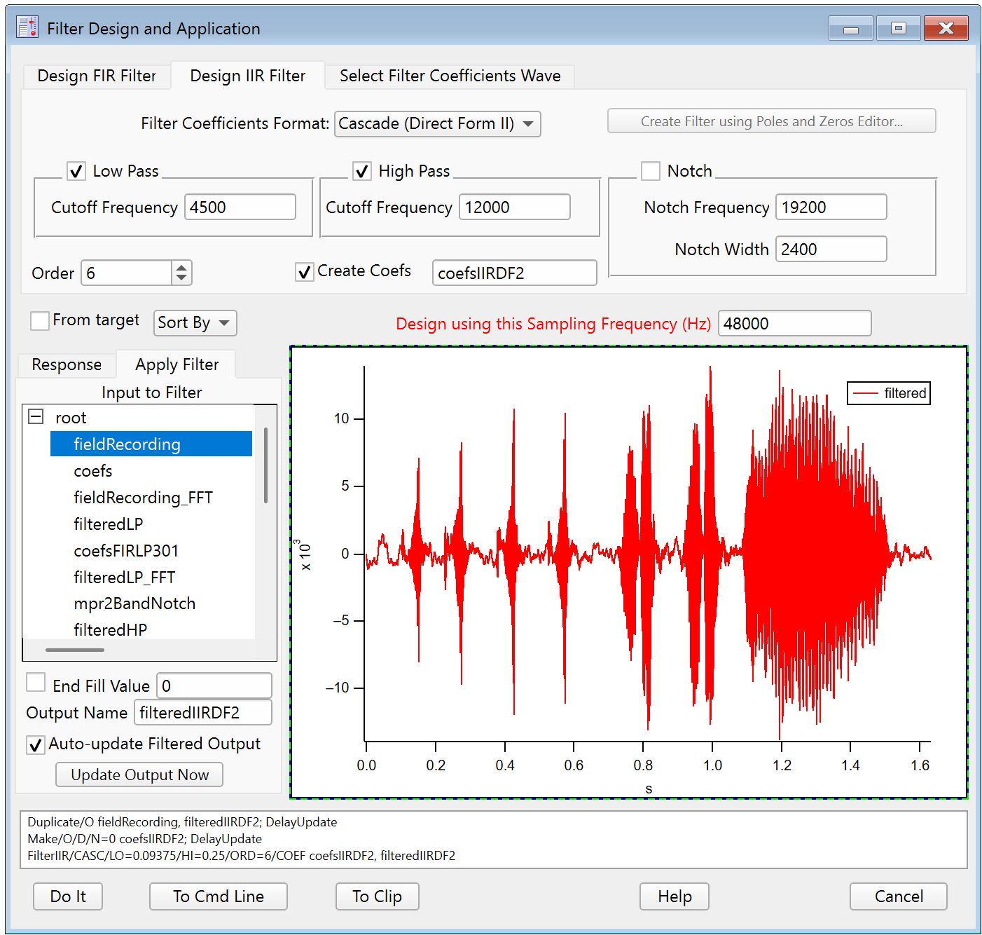
Applying an IIR Filter to Data

Click the Apply Filter tab to see the result of applying the designed filter to a waveform.

Select the input wave in the Input to Filter listbox and click either Auto-update Filtered Output checkbox or the Update Output Now button. This updates a preview of the filtered result.

Click Do It to create a final output wave in the current data folder. You can set the name of the final output wave in the Output Name field. Here we used filteredIIRDF2:

Evaluating a Digital Filter

The graph in the Response tab of the Filter Design and Application dialog is the most direct way to evaluate what the filter will do to an input waveform.

You can also graph the original data and filtered data for a detailed visual comparision.

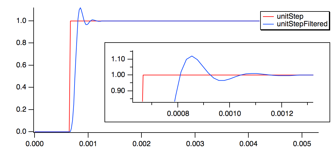
A useful technique, borrowed from electrical engineering, is to see how the filter responds to an ideal "unit step" waveform:

Make/O/N=256 unitStep = p >= 32                          // Create a unit step waveform suitable for causal IIR filters
CopyScales/P yourData, unitStep                          // Use the same sampling frequency as your data
Duplicate/O unitStep, unitStepFiltered                   // FilterIIR overwrites the input with the filtered result
FilterIIR/DIM=0/COEF=savedIIRDF1filter unitStepFiltered  // Apply a DF I filter to the unit step waveform
Display unitStep, unitStepFiltered                       // Observe the unfiltered and filtered waves

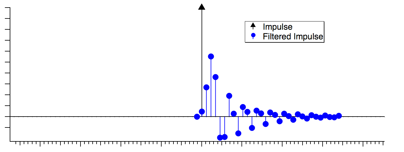
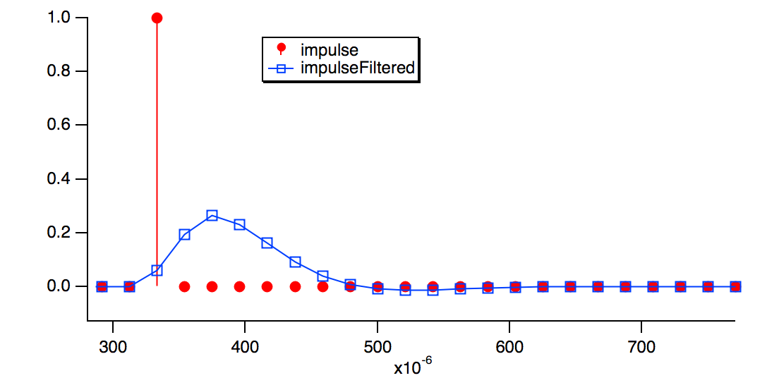
The next example shows how the filter responds to an ideal "unit impulse" waveform and display it's FFT magnitude, as the Filter Design and Application dialog does:

Make/O/N=2048 impulse = p == 16           // Create an impulse waveform suitable for causal IIR filters
CopyScales/P yourData, impulse            // Impulse is longer than step to improve FFT resolution
Duplicate/O impulse, impulseFiltered
FilterIIR/CASC/DIM=0/COEF=savedIIRDF2filter impulseFiltered // DF II implementation needs /CASC
Display impulse, impulseFiltered

FFT/MAG/DEST=impulseFiltered_FFT impulseFiltered   // Compute magnitude of impulse response
Display impulseFiltered_FFT
Display impulseFiltered_FFT                        // A logarithmic axis has the same shape 
ModifyGraph log(left)=1                            // as computing 20*log(response)

Applying an IIR Filter to Other Data

You can reuse a filter if you keep a copy of the design's output coefficients. For example:

Duplicate/O coefs, savedIIRfilter   // Keep a copy of the filter design.

You can apply the saved IIR filter to other data using the FilterIIR operation:

Duplicate/O otherData, otherDataFiltered              // FilterIIR overwrites the input with the filtered result
FilterIIR/DIM=0/COEF=savedIIRfilter otherDataFiltered // Apply saved filter to copy of otherData

You can also apply the saved IIR filter to other data using the Select Filter Coefficients Wave tab of the Filter dialog.

Rotate Operation

The Rotate operation rotates the data values of the selected waves by a specified number of points. When you choose Rotate, Igor displays the Rotate dialog.

Think of the data values of a wave as a column of numbers. If the specified number of points is positive the points in the wave are rotated downward. If the specified number of points is negative the points in the wave are rotated upward. Values that are rotated off one end of the column wrap to the other end.

The rotate operation shifts the X scaling of the rotated wave so that, except for the points which wrap around, the X value of a given point is not changed by the rotation. To observe this, display the X scaling and data values of the wave in a table and notice the effect of Rotate on the X values.

This change in X scaling may or may not be what you want. It is usually not what you want if you are rotating an XY pair. In this case, you should undo the X scaling change using the SetScale operation:

SetScale/P x,0,1,"",waveName  // replace waveName with name of your wave

Also see the example of rotation in Spectral Windowing.

For multi-dimensional wave rotation, see the MatrixOP rotateRows, rotateCols, rotateLayers, rotateChunks functions.

Unwrap Operation

The Unwrap operation scans through each specified wave trying to undo the effect of a modulus operation. For example, if you perform an FFT on a wave, the result is a complex wave in rectangular coordinates. You can create a real wave which contains the phase of the result of the FFT with the command:

wave2 = imag(r2polar(wave1))

However the rectangular-to-polar conversion leaves the phase information modulo 2π. You can restore the continuous phase information with the command:

Unwrap 2*Pi, wave2

The Unwrap operation is designed for 1D waves only. Unwrapping 2D data is considerably more difficult. See the ImageUnwrapPhase operation for more information