Igor Filter Design Laboratory (IFDL)

With the Igor Filter Design Laboratory you can design lowpass, highpass, bandpass, notch, differentiator, Hilbert, window, and arbitrary Finite Impulse Response (FIR) filters and "analog prototype" Infinite Impulse Response (IIR) filters.

The Compare Filters window overlays the responses of two filters for easy comparison.

You can export the filter coefficients as an Igor wave or as a text file in several formats.

You can incorporate all of IFDL into your existing Igor experiments, or incorporate only the portion needed to use an exported filter, simply by adding an #include line to one of your procedure windows. See Adding IFDL to an Existing Experiment.

IFDL is built into Igor 8

The IFDL operations Remez and FmaxFlat are built into copies of Igor 8 and later, and copies of the IFDL v4 procedures and this IFDL Help are pre-installed in the Igor Pro 10 Folder / Examples / IFDL v4 Procedures 'Welcome to IFDL.pxp' experiment.

Quick Review of Digital Filter Design

Before we turn you loose with IFDL, perhaps we should review a few things….

Digital filters generally come in two flavors: Finite Impulse Response (FIR) and Infinite Impulse Response (IIR) filters. IIR filters are new in IFDL version 4.

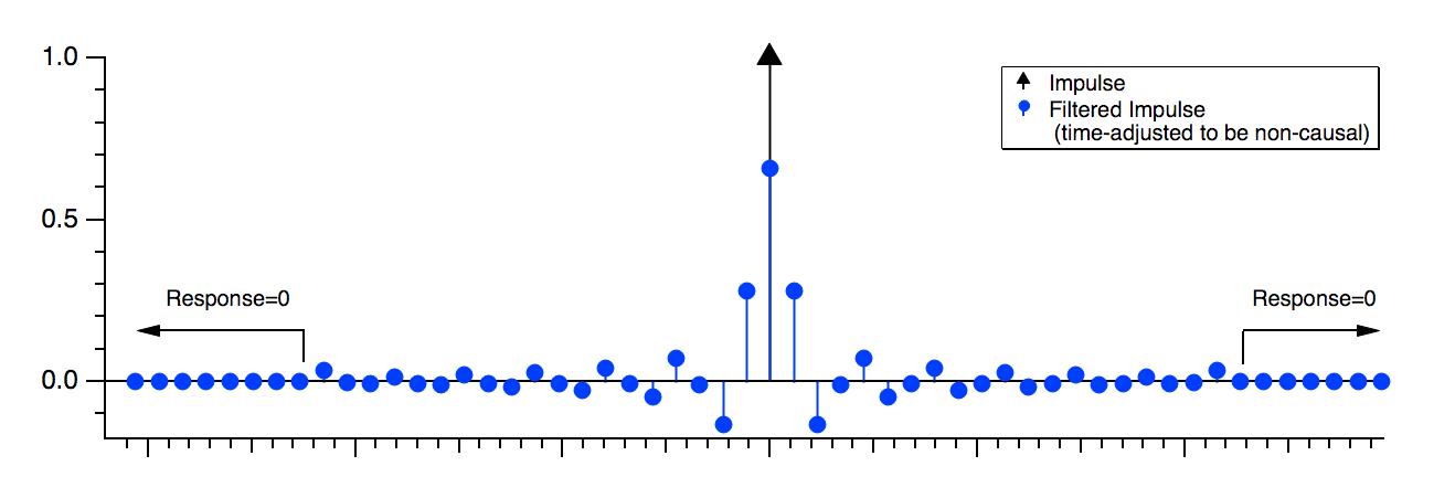
"Finite Impulse Response" means that the filter’s time-domain response to an impulse (or "spike") is zero after a finite amount of time:

Digital implementation of an FIR filter uses adders, multipliers, and delay elements connected without feedback (only feed-forward):

Where,

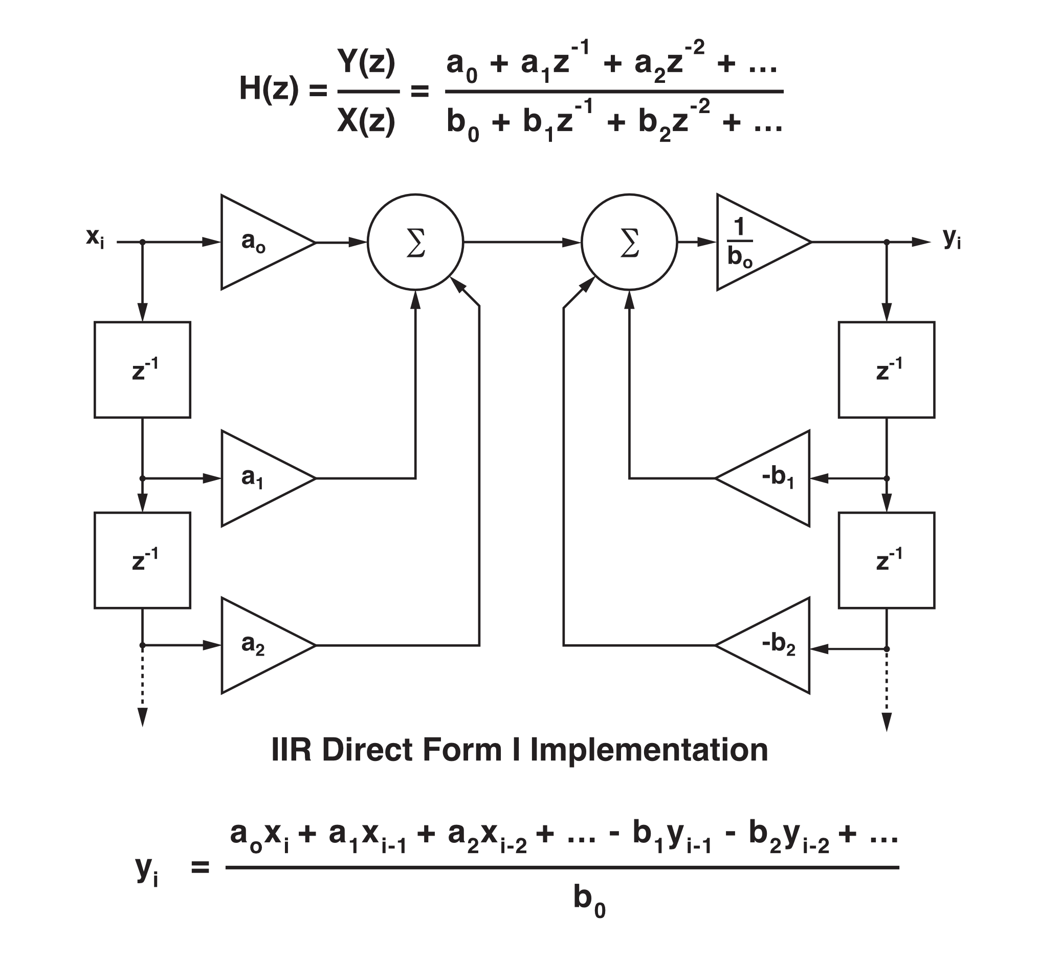
H(z) is the filter’s transfer function expressed as a Z transform,

y_i = … is the filter output expressed as a "difference equation",

x_i-n is the input signal delayed in time by n sampling intervals,

z^-n indicates a delay of n sampling intervals,

a₀, a₁, etc are multipliers,

and ∑ indicates summation.

The response of an IIR filter, however, continues indefinitely, as it does for analog electronic filters that employ inductors and capacitors:

Digital implementations accomplish this response by connecting delay elements in a feedback and feedforward configuration:

FIR Filter Design

A Finite Impulse Response (FIR) filter is a finite length, evenly spaced time series of impulses with varying amplitudes that is convolved with an input signal to produce a filtered output signal.

The impulse amplitudes are termed "weighting factors" or "coefficients". These impulse amplitudes are identical to the filter’s response to a unit impulse.

FIR filters are valued for their completely linear phase (constant delay for all frequencies), but they generally need many more coefficients than IIR filters do to achieve similar frequency responses. Consequently, physical digital realizations of FIR filters are usually more expensive than the corresponding IIR filter.

IIR Filter Design

A Infinite Impulse Response (FIR) filter is a set of coefficients or weights a₀, a₁, a₂,… and b₀, b₁, b₂… whose values and use depend on the digital implementation topology. Unlike the FIR filter, these coefficients are not the same as the filter’s response to a unit impulse.

The filter topology can be mathematically expressed by one or more "difference equations" that compute the output value y_i from previous input values x_i, x_i-1, x_i-2,… previous intermediate values w_i, w_i-1, w_i-2, and previous output values y_i-1, y_i-2,….

IIR filters can realize quite sophisticated frequency responses with very few coefficients. The drawbacks are non-linear phase, potential for numerical instability (oscillation) when realized using limited-precision arithmetic, and the indirect design methodology (frequency transformations of conventional analog filter methods).

IFDL implements two IIR topologies: the Direct Form I (see previous page) and the generalized Cascaded Bi-Quad Direct Form II:

The Cascaded Bi-Quad Direct Form II implementation works better than the Direct Form I when the filter order approaches 10 because it avoids computing differences of numbers with wildly different magnitudes. (A 10th order IIR filter uses 22 terms.)

Cascaded Bi-Quad Direct Form II also works better when limited-precision (say, 32-bit) hardware is used. It is a popular design for audio and video processing using 32-bit integer arithmetic.

Filter Design Goals

The goal of filter design is to determine the number and values of the filter coefficients which produce the desired frequency and phase characteristics.

You can specify desired filter characteristics using controls in IFDL’s "design graphs", and IFDL will:

• compute the required coefficients

• display the resulting filter characteristics

• (optionally) automatically apply the filter to your data

IFDL stores the computed filter coefficients in an ordinary Igor "wave".

The IFDL documentation refers to this representation of a filter as a "coefficients wave", a "filter coefficients wave", or a "filter wave".

In IFDL, the wave named "coefs" contains the filter coefficients for the most recently designed FIR filter.

The wave name "IIRCoefs" contains the most recently designed IIR filter.

You can save these filter coefficient waves under different names for export to another Igor experiment.

Nyquist Frequency

This Help occasionally refers to the "Nyquist frequency"; this term refers to one half of the sampling frequency.

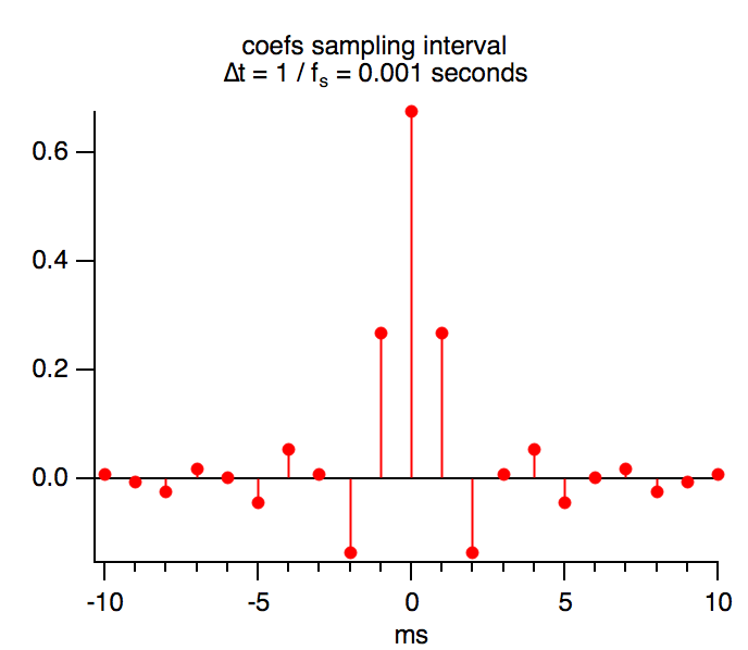
The sampling frequency determines the time interval between consecutive signal samples and between filter coefficient impulses. For example, a sampling frequency of 1000 Hz results in a Nyquist frequency of 500 Hz.

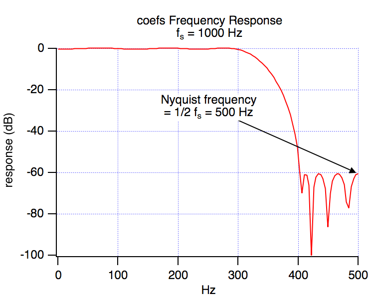
The Nyquist frequency is the highest frequency that can be adequately recovered from the sampled signal — higher frequencies will be erroneously recovered as "aliased" signals at some frequency below the Nyquist frequency. For this reason, the frequency response of an FIR filter is considered to end at the Nyquist frequency.

Consult a digital signal processing reference such as Elliot or Ramirez for a more thorough explanation of aliasing.

About Phase and Digital Filters

One of the primary reasons FIR filters are so useful is that it is trivial to produce zero-phase shift filters: simply keep the coefficients symmetric about the t=0 axis, and there is no phase shift (or completely linear phase shift caused by delaying the filter output).

All of the IFDL FIR filters produce zero-phase shift filters, except the Hilbert filter which is designed to produce a -90° phase shift.

IIR filters, on the other hand, do produce nonlinear phase shifts. This is a result of the filters’ recursive nature. The Bessel IIR filter was added to IFDL because it has nearly linear phase shift in the pass band.

IFDL Guided Tour

This Guided Tour will step you through most of the features of IFDL. We’ll skip some details that are covered in the IFDL Reference.

Follow along as we use IFDL to:

1. Add IFDL to an existing Igor experiment.

2. Design a notch filter and apply the filter to data already in the experiment.

3. Save the notch filter to compare with another filter, and for use in other experiments.

4. Design an arbitrary response filter to compare with the notch filter.

5. Compare the two filter designs.

6. Remove IFDL entirely from the Igor experiment.

7. Import the notch filter to another (new) experiment and use it without adding all of the IFDL procedures.

☞ The symbol to the left of this paragraph indicates that you should perform the operations described in the associated paragraphs. You should follow these steps carefully so that you will stay synchronized with the tour, and subsequent steps will work as expected. These instructions assume that you are familiar with the essentials of using Igor.

Adding IFDL to an Existing Experiment

Add IFDL 4 to any existing experiment by typing:

#include ":IFDL v4 Procedures:IFDL"

in any procedure window.

☞ To start the Guided Tour, open the Welcome to IFDL experiment.

Open Welcome to IFDL experiment

☞ Open the procedure window, and type #include ":IFDL v4 Procedures:IFDL" on its own line at the top of the window:

☞ Click the Compile button at the bottom of the window.

If you typed correctly, the compile button will disappear without show in any error dialog, and there will be a new IFDL menu in Igor’s menu bar.

☞ Close this procedure window (and any other procedure windows that are open).

Designing an FIR Lowpass Notch Filter

☞ Select ‘Set IFDL Parameters’ from the IFDL menu to display the SetIFDLParameters dialog.

☞ From the ‘get sampling frequency from:’ popup, choose the ‘myData’ wave that we’ve included in the Welcome to IFDL experiment.

IFDL uses the wave’s X scaling to set the sampling frequency used to design filters. This matches the range of the filter design parameters to the data’s frequency range. The myData wave’s X scaling corresponds to a sampling frequency of 5000 Hz.

You can also set the sampling frequency by choosing ‘_value entered manually_’ and entering "5000" directly in the ‘manual sampling frequency, Hz’ field.

☞ Use 1024 from the ‘frequency resolution (# of FFT values)’ popup menu for detailed frequency response graphs.

☞ Leave the other values at their defaults, and click ‘Continue’ to change the IFDL parameters. The IFDL control panel will be displayed:

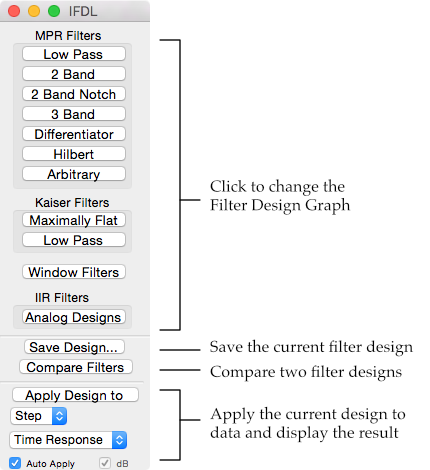
The IFDL panel provides access to most of IFDL’s features.

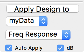
☞ Choose ‘myData’ from the popup menu near the bottom that is currently showing ‘Step’ (the wave selected here will have the current filter design automatically applied to it if the ‘Auto Apply’ checkbox remains checked).

☞ Choose ‘Freq Response’ from the popup currently showing ‘Time Response’ so that the result of the applied filter will be shown as a frequency response plot. Leave the dB (deciBel) checkbox checked.

☞ Click the ‘2 Band Notch’ filter design button to bring up one of the filter design graphs.

We chose this filter to remove a strong power-line component from the sample data, whose frequency response looks like this:

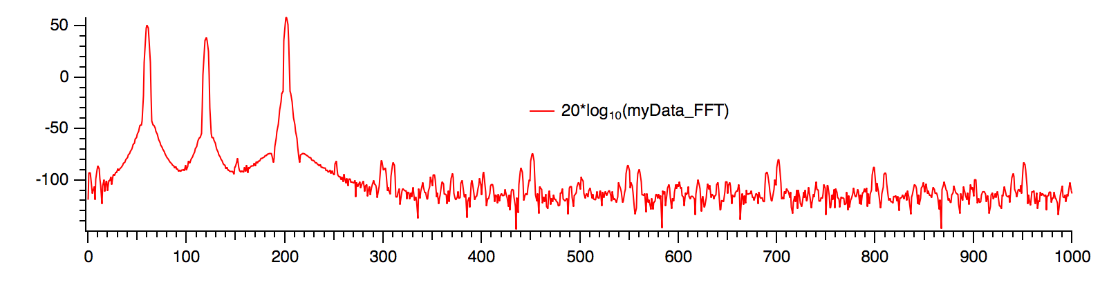
We will design a high-pass filter to recover the signal at about 200 Hz, with a notch at 60 Hz to reject the power-line signal’s fundamental frequency. We’ll set the high-pass cutoff frequency high enough to reject the 120 Hz harmonic of the power frequency, too.

☞ From the ‘Filter Type’ popup, choose ‘high pass’.

☞ Set the Notch Frequency to 60, or drag the vertical bar to the 60 Hz position.

☞ Set the End of First Band (the end of the reject band) to 150 Hz, and the Start of the Second Band (the start of the pass band) to 175Hz.

☞ Set the Number of Terms to 401 (this large number is needed to keep the passband response relatively flat).

☞ Leave the other values alone, and click Compute Filter:

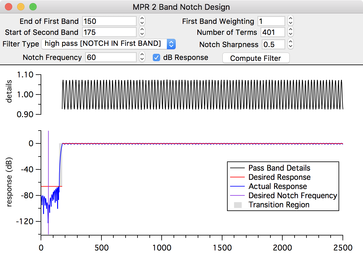
The frequency response of the designed filter is shown, in decibels, in the top graph. Notice the deep notch (-94 dB) at 60 Hz.

☞ Choose 'myData' from the IFDL Panel's Apply Design to popup, and choose 'Freq Response' to show the frequency response of the data and the filtered data displayed together in the ‘Filtered myData’ graph in decibels.

The 60 Hz and 120 Hz harmonic are absent from the filtered signal, and the 200 Hz signal remains.

☞ To see better detail, drag out a marquee in the "Filtered myData" window from 0 to 300 Hz, click inside and choose ‘Horiz Expand’:

Notice how the 60 Hz interference and the 120 Hz harmonic have been suppressed by as much as 70 dB. The signal to be recovered is barely affected.

☞ To see the time response of the filter, choose "Time Response" in the IFDL control panel, and click the ‘Apply Design to’ button. Use the marquee to horizontally expand the graph:

Here you can see that the filtered signal (solid line) doesn’t have the 60 Hz contamination that causes myData (dashed line) to wander.

Saving the Notch Filter Design

The current FIR filter is always stored in a wave named "coefs". New FIR designs will overwrite this coefs wave.

To keep the filter from being overwritten by another design, we must save it as an Igor binary wave under another name. This way we can use multiple filters in one experiment, such as when we compare filter designs or apply multiple filters.

☞ Click the ‘Save Design...’ button in the IFDL panel to get this dialog:

☞ To use the design within the current experiment, keep ‘Another Igor Wave’ selected and click ‘Continue’:

☞ IFDL proposes a name based on the design type. You can change this, but we’ll use the default. Click ‘Continue’.

You won’t see any change, but this wave will be available later so we can compare another design to it.

Now we’ll also save the design as an Igor Binary file for use in a new experiment:

☞ Click the ‘Save Design...’ button again, choose ‘Igor Binary File’ and click ‘Continue’:

☞ Click ‘Continue’ again to save the Igor binary wave file to disk:

This wave can be loaded into an Igor experiment and used as the filter coefficients with the FilterFIR operation.

Arbitrary FIR Filter Design

While most of the FIR filter design graphs work similarly to the 2 Band Notch design graph, the Arbitrary Filter design graph is a bit different. Follow along as we use it to try to improve on the 2 Band Notch filter we’ve already designed.

☞ Click on the ‘Arbitrary’ button in the IFDL control panel:

note

For legibility’s sake, we set the axis range of the responseLeft axis to autoscale using the "Nice + inset data" setting in the Set Axis Range dialog in the Graph menu.

We’ll design a wide-notch filter, which will require 3 bands (one reject and two pass bands).

Desired Response Trace Preset

The first task is to create the desired response curve. The Preset controls help you get started.

☞ Click on the ‘Preset Bands’ SetVariable control until it reads "3".

☞ Click the ‘Preset Bands’ button.

☞ Click the ‘Edit Response’ button.

Adjusting the Desired Response Trace

The bands are distributed evenly over the Nyquist frequency range. We’ll move the reject band to span 60 and 120 Hz, allowing signals near 0 Hz and 200 Hz to pass.

☞ Drag the vertical response line currently at 800 Hz left until the X: readout indicates about 40 while holding down the Shift and Ctrl keys.

☞ Drag the remaining vertical response line at 1700 Hz down to about 140 Hz.

☞ Click the ‘Finish Response’ button:

To Weight or Not to Weight...

Weighting values are used to give higher importance to one region of the response curve. We’ll use uniform weighting to start out with.

☞ Click the ‘None’ weighting button. This sets all the weighting values to 1.

Deleting Transition Regions

The shaded transition regions indicate frequencies where we expect the response to change from a reject band to a pass band, so we don’t constrain the response to a particular value. Using a transition region allows the filter design algorithm more freedom to optimize the response in places where we do care about what the response is.

These transition bands are in the wrong place. The Arbitrary Filter Design graph can’t move the transition regions, but you can add or delete them using the marquee.

We’ll delete the existing transition bands and add more precise ones after zooming in on the low frequencies.

☞ To delete the transition regions, click to the left of 500 Hz, and drag a marquee out that encompasses the 500 Hz to 2250 Hz range, click inside the marquee, and choose ‘Remove_Transition_Region’ from the resulting popup menu:

☞ Expand the low frequencies by dragging out a marquee that starts at about 20 Hz and ends near 160 Hz, clicking inside the marquee, and choosing ‘Horiz Expand’ from the popup menu (or use the Set Axis Range dialog in the Graph menu):

☞ (Optional) With the low frequencies expanded out, you might take the opportunity to adjust the desired response trace more accurately.

Adding Transition Regions

Now we’ll add transition regions around where the response changes between pass band and reject band.

☞ Drag out the marquee from 30 Hz to 50 Hz to enclose the 40 Hz vertical response line without including the 60 Hz region, click inside the marquee, and choose ‘Add_Transition_Region’:

☞ Repeat for 130 Hz - 150 Hz:

We’ve specified the desired response: a reject band encompassing the 60 Hz and 120 Hz interference signals, and two pass bands that preserve the constant (0 Hz) level, the signal frequency (200 Hz), and most other frequencies.

Filter Terms - How Many is Enough?

The default Filter Terms setting of 41 is for filters with large bands, not the narrow ones we’re creating. (If you try 41 terms, choose ‘Autoscale Axes’ from the Graph menu to see the entire response to assess the result.)

An odd number of terms is required because it eliminates phase shift in the filtered result. Since we’ll be comparing this filter with the 2 Band Notch filter, we’ll use the same number of terms.

☞ Change the Filter Terms value to 401.

☞ Click the ‘Compute Filter’ button:

This shows the gain of the computed filter over the 0-165 Hz range.

note

The responses you obtain will be slightly different, depending on the actual desired response and transition regions values you entered.

Critiquing the Designed Filter

At first glance, the filter seems quite adequate: the reject band is near zero and the the passband (what little we can see of it) has very little ripple. Let’s take a closer look.

☞ Check the ‘dB Response’ checkbox. We also set the response axis range to about -80 to 10 and turned on the grid for the responseLeft axis:

The rejection in the 50 to 130 Hz region is about -30 dB. This corresponds to a gain of

10^^(-30/20) = 3.2%. For some applications this might be good enough, but we’ll attempt to do better.

☞ To see the response over the entire frequency range, choose ‘Autoscale Axes’ from the Graph menu.

☞ Uncheck the dB Response checkbox:

The passband does indeed have a nice equiripple response very close to unity gain. To measure the pass band response, we need to zoom in.

☞ Use the Set Axis Range dialog to set the range of the responseLeft axis to vary from a minimum of 0.95 to a maximum of 1.05:

Now we can see that the gain of our computed filter in the passband is between 0.98 and 1.02 (or +/- 0.17 dB).

Improving the Design

The reject band suppresses the 60 Hz and 120 Hz interference signals by about -30 dB (3% gain). We’d like to improve that to about -50 dB (0.3% gain).

There are two usual methods used to improve a filter:

• Increase the number of filter terms. This usually works by reducing the errors (usually also increasing the number of ripples in the response).

• Use weighting values. Larger weighting values improve accuracy in one part of the frequency range by reducing accuracy in the remaining frequency range. This method keeps the same number of filter terms.

Improving the Design by Increasing the Number of Terms

Let’s drastically increase the number of terms and see what happens:

☞ Change the Filter Terms value to 701.

☞ Click ‘Compute Filter’.

(Sometimes this very large number of terms will cause the filter design algorithm to fail; try an intermediate value like 601 if you get an error dialog.)

☞ Use the marquee or Set Axis Range dialog to zoom in on the 20 Hz - 160 Hz range.

☞ Click the ‘dB Response’ checkbox and set the responseLeft axis range to min -80 and max of 0:

The response in the reject band is flatter and much deeper, about -55 dB!

Checking the new response over the entire frequency range shows that the ripple is almost zero (less than 0.02 dB).

We’re done if the increased number of terms is no problem for us (for instance, we’re not going to implement the filter in hardware, where more terms usually are either more expensive or possibly too slow for realtime conversions).

Next we’ll show you how to improve the filter while using the same number of terms.

Improving the Design with Weighting

You can force the design algorithm to give higher priority to portions of the desired response by assigning a higher weighting value to that frequency range. The default weighting value is 1.0, the value applied to all frequencies when you click the ‘None’ weighting button.

We will assign a higher weighting value to the reject band of frequencies. First, change the number of filter terms back to 401.

☞ Enter 401 in the ‘Filter Terms’ control.

☞ Click ‘Compute Filter’ to get the original filter response.

There are two ways to assign weighting values:

• Click the ‘Edit Weighting’ button, and edit the weighting trace directly.

• Use the marquee to set a range to a constant value.

We’ll use the marquee:

☞ Drag out a marquee over the range of approximately 40 Hz to 140 Hz, click in the marquee and choose ‘Set_Weighting_Value’:

☞ Enter 10 in the resulting dialog and click ‘Continue’.

☞ Click ‘Compute Filter’:

The rejection at 60 and 120 Hz has been improved to -45 dB (from -30 dB).

Checking the passband response shows that the variation has increased to +/- 0.4 dB (from +/- 0.17 dB). The weighting has traded greater accuracy in the reject band for a slight loss of accuracy in the pass bands. This tradeoff is fairly typical of filter design.

Let’s see how this filter compares to the 2 Band Notch filter we designed earlier.

Comparing Filter Designs

The current design is always stored in the Igor binary wave named "coefs". This contains the design for the Arbitrary Filter we just finished. (We could save coefs into another Igor Binary wave so that it won’t be overwritten by a later design.)

We saved the 2 Band Notch filter design earlier into a wave named "mpr2BandNotch".

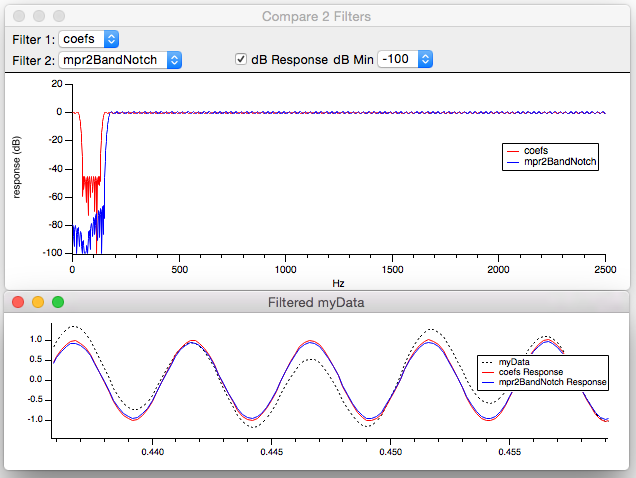
We’ll use the Compare Filters graph to compare these two designs.

☞ Click the ‘Compare Filters’ button in the IFDL control panel.

☞ Choose ‘mpr2BandNotch’ from the Filter 2 popup menu.

The frequency responses of both filters are displayed, and if the the ‘Auto Apply’ checkbox in the IFDL panel is still checked, the time-domain responses of applying each filter to myData are also displayed in a 'Filtered myData' graph:

Both filters recover the signal adequately.

By expanding the low frequencies of the Compare 2 Filters graph, you can see that our 2 Band Notch rejects the noise more completely, while the arbitrary filter can pass more frequencies (including the often-important 0 Hz):

You can also simultaneously observe the passband response using the ‘Apply Filters to’ button:

☞ Choose ‘Impulse’ from the IFDL control panel’s data wave popup menu (just below the ‘Apply Filters to’ button).

☞ Choose ‘Freq Response’ from the IFDL control panel popup menu below ‘Impulse’.

☞ Click the ‘Apply Filters to’ button.

☞ Expand the passband frequencies with the marquee or the Set Axis Range dialog:

You can see that the arbitrary response filter has slightly lower passband error.

Another helpful comparison is to observe the frequency response of the data before and after filtering.

☞ Choose ‘myData’ from the IFDL control panel’s data wave popup menu.

☞ Choose ‘Freq Response’ from the IFDL control panel popup menu.

☞ Click the ‘Apply Filters to’ button.

☞ Expand the low frequencies with the marquee or Set Axis Range dialog:

Here you see the 2 Band Notch filter more thoroughly rejecting the 60 Hz and 120 Hz interference than the Arbitrary filter.

Entirely Removing IFDL from an Experiment

We’ve already saved the 2 Band Notch filter to a file for later use. We’ll abandon the arbitrary filter and show you how to remove IFDL completely from the experiment:

☞ Choose ‘Delete All IFDL Data’ from the IFDL menu:

You will see two dialogs asking you to confirm the deletion of data:

☞ Click ‘Yes’ in each of them.

Under unusual circumstances you might be using the root:WinGlobals data folder, in which case you should answer ‘No’ to the second dialog (there is no harm in doing so).

You have now removed all the IFDL waves, strings, variables, and data folders from the experiment, except for some waves that IFDL left in your current data folder (the saved filters, coefs, and filtered signal results). You may wish to remove these waves:

☞ Choose ‘Data Browser’ from the Data menu.

☞ Drag out a marquee that intersects all waves you no longer want.

☞ Click the ‘Delete...’ button in the Data Browser, and ‘Delete’ in the resulting dialog:

☞ Close the Data Browser.

Now we’ll remove the IFDL procedures.

☞ Open the main procedure window by pressing Ctrl+M.

☞ Delete the #include ":IFDL v4 Procedures:IFDL" line we originally added.

☞ Save the experiment (to prepare for its use in the next section).

IFDL is completely removed from the Welcome to IFDL experiment.

Importing a Filter into an Experiment

Now suppose you have saved some filters as Igor binary waves to disk, and you want to apply a filter to your data in another experiment. You could add all of the IFDL procedures to your experiment, as we did to the Welcome to IFDL experiment, but we’ve provided a smaller procedure that compiles faster.

IFDL ships with a standalone procedure file you can include in your experiment to apply a filter to your data.

Follow along as we:

• Import the 2 Band Notch filter we saved earlier.

• Add the ‘IFDL Apply Filter’ procedure to an Igor experiment.

• Apply the 2 Band Notch filter to some data.

• Remove the added procedure and imported filter.

☞ If not still open, open the modified Welcome to IFDL experiment you saved earlier.

Now we’ll create some data to be filtered.

☞ Choose the ‘MakeMyData’ macro from Igor's Macros menu.

☞ Choose ‘New Graph’ macro from the Windows menu, and select myData.

This is the same myData wave we used when designing the filters, but let’s pretend it is your actual data from your own experiment.

Importing the Filter

☞ Choose ‘Load Igor Binary...’ from the Data menu’s ‘Load Waves’ submenu:

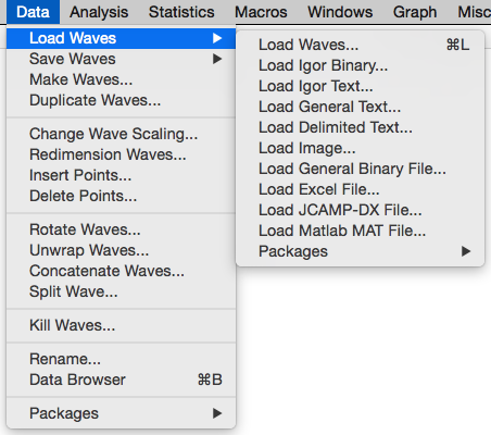
☞ In the resulting dialog, select the ‘mpr2BandNotch.bwav’ file we saved earlier.

☞ If you get the ‘Copy or Share Wave?’ dialog, choose Copy and click OK.

Applying the Filter

There are several ways to apply a filter to your data.

The simplest way is to use the Filter Design and Application Dialog in Igor 6 and later and the Select Filter Coefficients Wave tab.

☞ Select the saved filter design wave in the Select Filter Coefficients Wave tab of the Filter Design and Application Dialog.

☞ Select the wave to be filtered from the Apply Filter tab below.

Another way is described in Adding the IFDL Apply Filter Procedure, below.

You can also apply a filter by writing an FilterFIR or FilterIIR command:

For example, to apply a saved FIR filter to new data using the FilterFIR command either on the command line or in a user-defined macro or function:

Duplicate/O otherData, otherDataFiltered	// FilterFIR overwrites the input with the filtered result.
FilterFIR/DIM=0 /COEF=mpr2BandNotch.bwav otherDataFiltered	// Apply filter to copy of otherData

Adding the IFDL Apply Filter Procedure

☞ Open the procedure window, and type #include ":IFDL v4 Procedures:IFDL Apply Filter" on its own line at the top of the window:

☞ Click the Compile button.

There will now be a new Apply IFDL Filter To Data item in the Analysis menu.

☞ Choose the ‘Apply IFDL FilterToData’ item.

☞ Select the mpr2BandNotch filter in the ‘FIR or IIR filter coefficient wave’ popup.

Leave the ‘FIR filtered output’ popup set to "not delayed" We would choose "delayed" if we wanted to delay the filtered output. See Digital Filtering for more information.

☞ Click ‘Continue’.

☞ In the resulting graph of data and filtered data, set the bottom axis range from 0.50 to 0.55 to see the detailed results:

Removing the IFDL Apply Filter Procedure and Filter

To remove the IFDL procedure, delete the #include ":IFDL v4 Procedures:IFDL Apply Filter" line from the procedure window.

To delete the filter wave mpr2BandNotch, use the Kill Waves dialog or the Data Browser’s Delete button.

End of Guided Tour

We’ve now shown you how to add, use, and remove IFDL with one of your own existing experiments, and how to import and apply designed filters in other existing experiments.

There are other IFDL features you haven’t used in this Guided Tour, but they all work in a similar fashion.

The remaining topics describe IFDL features in detail without guiding you through the steps of using them.

IFDL Reference

The usual process for using IFDL is:

1. Add the IFDL procedures to your experiment.

2. Set the sampling frequency and other IFDL parameters.

3. Design a filter while observing how it affects your data.

4. Save the filter coefficients as an Igor binary file for later use.

Optional steps follow:

5. Import the filter into an experiment containing data to be filtered.

6. Add the IFDL Apply Filter procedure to your experiment.

7. Apply the filter to your data.

A step-by-step walkthrough of this process that covers the basic features of IFDL is provided in IFDL Guided Tour.

This IFDL Reference describes the features of IFDL in more detail.

Adding IFDL to an Existing Experiment

After installing the IFDL extension and procedures (see "Installing IFDL" in the IFDL experiment IFDL / IFDL Guided Tour Help), you can add IFDL to any existing experiment by typing:

#include ":IFDL v4 Procedures:IFDL"

in any procedure window, and clicking the Compile button at the bottom of the procedure window.

If IFDL is correctly installed and you typed correctly, the compile button will disappear without producing any error dialog, and there will be an IFDL menu in Igor’s menu bar.

To remove IFDL from an experiment, see "Entirely Removing IFDL from an Experiment" in the IFDL Guided Tour.

IFDL Lite

If you have an already-designed filter you want to apply to your data, you can instead type:

#include ":IFDL v4 Procedures:IFDL Apply Filter"

This adds only the Apply IFDL Filter To Data macro to your Analysis menu, rather than adding the entire IFDL menu.

The primary advantage is that fewer procedure files will be opened so that your procedures will compile somewhat faster, and fewer IFDL-related waves, variables, strings, data folders, graphs, and panels will be created in your experiment.

For more information, see Adding the IFDL Apply Filter Procedure".

You will need to import your filter wave into the experiment, too. See Importing the Filter.

The IFDL Menu

Here is what the IFDL menu items do:

Set IFDL Parameters...	Brings up the Set IFDL Parameters dialog to set sampling frequency and other globally applicable filter and IFDL values. Displays the IFDL control panel if not already shown.
Filter Designs	Displays the IFDL control panel. If IFDL has not been initialized, it first brings up the Set IFDL Parameters dialog.
Normalize Design Coefficients...	Sets the filter gain to exactly 1.0 at a given frequency.
Save Design	Saves the current filter design in a variety of formats. Same as the ‘Save Design...’ button in the IFDL control panel.
Compare 2 Filters	Compares the frequency responses of two filters saved in Igor binary waves. Same as the ‘Compare Filters’ button in the IFDL control panel.
Sine Sweep Test Signal...	Creates an Igor binary wave that sweeps a sine wave over a range of frequencies. A useful signal to demonstrate a filter’s response in the time domain.
Two Tones Test Signal…	Creates an Igor binary wave that is the sum of two sine waves. A useful signal to demonstrate a filter’s response in the frequency domain.
Apply Filter...	Applies a filter to data stored in an Igor binary wave. Same as the ‘Apply Filter to’ button in the IFDL control panel.
Close All IFDL Windows	Closes all windows (graphs, panels, layouts) created by IFDL. Does not delete any data.
Delete All IFDL Data	Closes all IFDL windows and deletes all the IFDL data stored in the IFDL data folder(s). Some IFDL-created data remains in the current data folder, notably the ‘coefs’ and ‘IIRCoefs’ Igor binary waves which contain the filter coefficients.

Setting the IFDL Parameters

IFDL needs to know what frequency your data will be sampled at, because a Finite Impulse Response filter designed for one sampling rate will produce incorrect results when applied to a signal sampled at a different rate (however, see Normalized Frequencies, below.)

Select ‘Set IFDL Parameters...’ from the IFDL menu to set the frequency at which your data will be sampled at, and other IFDL values:

After you make your selections and click Continue, IFDL will:

• Show the IFDL control panel if it isn’t already showing.

• If a filter design graph is showing, the current filter will be recomputed with the changed parameters.

The dialog parameters are:

• ‘get sampling frequency from:’ determines whether the sampling frequency is set automatically to match the selected wave’s X scaling, or whether it is entered manually in the ‘manual sampling frequency, Hz’ field.

  Selecting a wave from this popup sets the filter sampling frequency to 1/Ʈx(selectedWave). Both the signal and the designed filter coefficients will be represented by impulses separated in time by deltax(selectedWave).

• ‘sampling frequency, Hz’ determines the X scaling of filters and filtered signals. In this Help, the sampling frequency is sometimes referred to as fs. A sampling frequency of 5000 Hz, for example, would result in the selected filter’s X scaling being set to 0.002 seconds between adjacent points:

  

  By default, the dialog shows f_s = 1 Hz, corresponding to X scaling of 1 second between adjacent points.

Normalized Frequencies

It is common to design a filter using "normalized frequencies", where all frequencies are expressed as a fraction of the sampling frequency. To use normalized frequencies in IFDL, leave f_s = 1 Hz, and interpret "Hz" to mean "fraction of sampling frequency".

Changing a Filter’s Sampling Frequency

You can change the sampling frequency of the current design by choosing Set IFDL Parameters from the IFDL menu and altering the sampling frequency. This will scale the current design to the new frequencies. All frequency-based parameters will be scaled to the same percentage of the sampling frequency.

For example, if the filter originally had a sampling frequency of 100 Hz, and an end-of-first-band frequency value was 20 Hz (20% of f_s) changing the sampling frequency to 300 Hz will alter the end-of-first-band frequency to 20% of 300 Hz, or 60 Hz.

When you change the sampling frequency, IFDL forcibly re-computes the filter coefficients and displays the changed responses.

• ‘frequency resolution (FFT values)’ determines how many values are computed for the frequency response graphs. With a frequency resolution value of 1024, the displayed frequency resolution will be 1/1024th of the Nyquist frequency.

  This frequency resolution setting does not affect the filter coefficients in any way.

  Continuing the example above, if f_s = 5000 Hz, the frequency resolution of the FFT results will be 2500 Hz/1024 = 2.4 Hz (remembering that the Nyquist frequency is half the sampling frequency).

• ‘quantization type’ is a popup which selects the default filter coefficient number representation simulated by IFDL.

  "floating point" represents the coefficients as a floating point number. This means that the FIR filters we design are intended to be implemented using software or hardware to multiply and sum the digitized input signal using floating point representations.

  "fixed point" selects scaled integer representations.

• ‘bits of quantization’ is the number of bits in the mantissa of floating point filter coefficients. For fixed-point quantization, this is the number of bits in each integer filter coefficient. 53 is the maximum number of bits supported by IFDL. This corresponds to double-precision floating point number in IEEE format.

Filter Delay

• ‘FIR output timing’ determines the timing relationship between the input signal and the filtered output signal produced by the filter. Here it is set to ‘in phase with input’, so that the filtered output is not delayed with respect to the filter’s input.

  IFDL implements ‘in phase with input’ by advancing the timing of the filter coefficients by one half of the filter length into the future. Coefficients associated with negative (future) time are applied to input signal samples that haven’t arrived yet.

  

  This time axis labeling is backwards from the normal convention of increasing time left to right, where "future" samples are off the graph to the right. The reversal is the result of the convolution equation:

$$\displaystyle { Filtered }(t)=\sum_{i=-\left(\frac{N-1}{2}\right)}^{\frac{N-1}{2}} {Signal}(t+i) \bullet {Filter}(-i)$$

The equation shows that signal samples displaced in a positive direction (future-ward samples) are multiplied with filter coefficients with negative x values (future-ward coefficients).

"In phase with input" timing makes comparison of the input and filtered signal easier, and is appropriate when the input signal is stored or buffered in memory before the filtering is performed.

The other popup choice is ‘delayed (causal)’, which means the filtered response is delayed with respect to the input signal. This second choice is appropriate when the input signal is not stored in memory before the filtering is performed (i.e., the filtering is performed in "real-time").

<img src="MD_images/Igor Filter Design Laboratory/Setting_the_IFDL_Paramete_5.png" width="50%"/>

• ‘IFDL legend font size (points)’ does not affect the filter at all; it simply allows you to shrink or expand the various legends that IFDL automatically puts in the graphs.

  The new font size will be used when IFDL next creates or modifies an automatically generated legend.

FIR Filter Designs

Choosing the ‘Filter Designs’ IFDL menu item displays the IFDL control panel, which provides access to most of IFDL’s features.

note

If IFDL has not yet been initialized, the Set IFDL Parameters dialog is shown, first.

The first group of buttons will bring up a "filter design graph": an Igor graph with controls in it to set the parameters for the kind of filter being designed.

Only one filter design graph may be displayed at a time.

See Filter Design Graphs for information about each filter design graph.

Click the ‘Save Design...’ button to save the current filter coefficients in the "coefs" wave as another Igor wave or to a file.

You can save the coefficients as an Igor binary wave in the current experiment, or as a file in binary or text formats. See Save Design, later in this help for more details.

Click the ‘Compare Filters’ button to bring up a graph that compares two filter designs. The filter coefficients must be stored in Igor binary waves, one of which can be the most recently computed filter stored in "coefs" wave.

The last group of controls apply the current filter stored in the "coefs" or "IIRCoefs" wave to data selected in the top popup menu, and displays the result in a separate "Filtered dataWave" graph.

The top popup menu shows data waves already in the current experiment and two special waves named "Impulse" and "Step" so that you can easily evaluate the impulse and step response of a filter:

Use the bottom popup menu to choose between frequency response or time-domain response.

These Filtered dataWave graphs are updated:

• When you click the ‘Apply Design to’ button.
• (if the ‘Auto Apply’ checkbox is checked) whenever a filter design is computed.
• (if the ‘Auto Apply’ checkbox is checked) whenever a different filter is selected in the Compare Filters graph).

Normalize Design Coefficients...

Normalizing a filter adjusts the scaling of all coefficients by a factor, k, so that the filter’s magnitude response at a particular frequency is 1.0. You might choose to normalize a filter at an important signal frequency; perhaps 0 Hz to preserve D.C. response.

‘Normalize Design Coefficients’ can be used to adjust the filter coefficients by a scale factor to normalize the filter response at a particular frequency or at the maximum amplitude frequency.

The computed scale factor k is printed in the command history window.

note

You should immediately use Save Design on the normalized filter. When you re-compute the filter for any other reason, the normalization is lost.

The dialog parameters are:

• ‘Normalization frequency, or <0 for peak frequency’ is the frequency at which the current filter’s gain is normalized to 1.0. Enter the frequency between 0 and the Nyquist frequency, or enter "-1" to normalize the filter’s maximum response to 1.0.

• ‘Quantize the coefficients?’ asks you whether to quantize the normalized filter to the number of bits specified in the ‘Set IFDL Parameters’ dialog.

Quantizing a filter will limit how accurately the filter can be normalized. This is usually noticeable only when there are many filter terms and relatively few bits (say, 100 terms and 16 bits), or when an IIR filter uses the Direct Form I implementation.

Save Design

The current FIR filter is always stored in a wave named "coefs", and the current IIR filter is stored in a wave named "IIRCoefs". Computing new designs will overwrite these waves.

To preserve the result of one design for comparison with another design result — or to use the filter in another experiment — you can save the current filter wave in a variety of formats using either the Save Design submenu of the IFDL menu or the ‘Save Design...’ button in the IFDL control panel:

note

Saving the filter coefficients doesn’t actually save all the design parameters, just the coefficients which are a result of using those parameters, and some basic parameters in the wave's note.

The filter design parameters for each design graph are saved in the experiment in which the filter was designed, in waves, variable, and strings within the root:Packages:WM_IFDL: data folder.

Descriptive Text File

‘Descriptive Text File’ creates a text file listing the filter coefficients. The format is different for FIR and IIR filters.

The FIR format follows Momentum Data Systems Inc’s FIR filter coefficient file format.

Here is an (abbreviated) example of the MDS file format:

FILTER COEFFICIENT FILE
FIR DESIGN
28         /* number of taps in decimal */
001c       /* number of taps in hexadecimal*/
24         /* number of bits in quantized coefficients(decimal) */
0018       /* number of bits in quantized coefficients(hexadecimal)*/
0          /* shift count in decimal */
0000       /* shift count in hexadecimal */
    -93424 FFFE9310   /* coefficient of tap 0  */
    -171217 FFFD632F  /* coefficient of tap 1  */
    -33496 FFFF7D28   /* coefficient of tap 2  */
    139245 00021FED   /* coefficient of tap 3  */
    114123 0001BDCB   /* coefficient of tap 4  */
    ...
    114123 0001BDCB   /* coefficient of tap 23 */
    139245 00021FED   /* coefficient of tap 24 */
    -33496 FFFF7D28   /* coefficient of tap 25 */
    -171217 FFFD632F  /* coefficient of tap 26 */
    -93424 FFFE9310   /* coefficient of tap 27 */
-1.113699655979872e-02 BC3677F300000000 /* coefficient of tap 0  */
-2.041061595082283e-02 BCA7342A00000000 /* coefficient of tap 1  */
-3.993035294115543e-03 BB82D80200000000 /* coefficient of tap 2  */
1.659924909472466e-02 3C87FB2600000000  /* coefficient of tap 3  */
1.360450591892004e-02 3C5EE56F00000000  /* coefficient of tap 4  */
...
-1.996348612010479e-02 BCA38A7700000000 /* coefficient of tap 22 */
1.360450591892004e-02 3C5EE56F00000000  /* coefficient of tap 23 */
1.659924909472466e-02 3C87FB2600000000  /* coefficient of tap 24 */
-3.993035294115543e-03 BB82D80200000000 /* coefficient of tap 25 */
-2.041061595082283e-02 BCA7342A00000000 /* coefficient of tap 26 */
-1.113699655979872e-02 BC3677F300000000 /* coefficient of tap 27 */

You can change the format by editing the ‘DescriptiveTextFile’ procedure in the IFDL.ipf procedure file.

The IIR formats are different, and depend on the IIR filter implementation.

Here is an example of the Direct Form I implementation format:

FILTER COEFFICIENT FILE
IIR DIRECT FORM 1 DESIGN

Chebyshev low pass; 2 bands
Band	Start Freq (Hz)	End Freq (Hz)
1           0           1250    (pass band)
2           1250        2500    (reject band)
(end)

Z-plane poles:
	0.5509033687686493 + j    -0.3350683608090418
	0.5509033687686493 + j     0.3350683608090418
	0.2330879372966871 + j    -0.7665180267265226
	0.2330879372966871 + j     0.7665180267265226
	0.0043816972451698 + j    -0.9393540340690545
	0.0043816972451698 + j     0.9393540340690545

Z-plane zeros:
	-1.0000000000000000 + j     0.0000000000000000
	-1.0000000000000000 + j     0.0000000000000000
	-1.0000000000000000 + j     0.0000000000000000
	-1.0000000000000000 + j     0.0000000000000000
	-1.0000000000000000 + j     0.0000000000000000
	-1.0000000000000000 + j     0.0000000000000000

53 bit floating point mantissa

Delay    Numerators                Denominators
0   	0.00963112711906433        1
1   	0.0577867664396763         -1.57674586772919
2   	0.144466906785965          2.46742701530457
3   	0.192622542381287          -2.29841303825378
4   	0.144466906785965          1.66127419471741
5   	0.0577867664396763         -0.797427535057068
6   	0.00963112711906433        0.235488712787628

output[i]= (1/denominator[0]) * ( numerator[0]*input[i] + ... numerator[6]*input[i-6] - 
denominator[1]*output[i-1] - ... denominator[6]*output[i-6] )

The last line of the file (which is shown wrapped here) is a reminder of how the numerator and denominator coefficients of the filter are used in the "difference equation" for the Direct Form I implementation.

Here is an example of the same filter implemented as a Cascaded Bi-Quad Direct Form II filter:

FILTER COEFFICIENT FILE
IIR CASCADE DIRECT FORM II DESIGN

Chebyshev low pass; 2 bands
Band	Start Freq (Hz)	End Freq (Hz)
1            0          1250    (pass band)
2            1250       2500    (reject band)
(end)

Z-plane poles:
    0.0043816972451699 + j    -0.9393540340690545
    0.0043816972451699 + j     0.9393540340690545
    0.2330879372966871 + j    -0.7665180267265226
    0.2330879372966871 + j     0.7665180267265226
    0.5509033687686492 + j    -0.3350683608090419
    0.5509033687686492 + j     0.3350683608090419
Z-plane zeros:
    -1.0000000000000000 + j     0.0000000000000000
    -1.0000000000000000 + j     0.0000000000000000
    -1.0000000000000000 + j     0.0000000000000000
    -1.0000000000000000 + j     0.0000000000000000
    -1.0000000000000000 + j     0.0000000000000000
    -1.0000000000000000 + j     0.0000000000000000

56 bit floating point mantissa

3 cascaded sections
    |------------------------------ numerators ------------------------------|       |------------------------------ denominators ---------------------------|
sec         a0                      a1 (z^-1)                  a2 (z^-2)                     b0                        b1 (z^-1)                 b2 (z^-2)    
 1   0.00963112525641918        0.0192622505128384         0.00963112525641918        1                          -0.00876339431852102       0.882405281066895        
 2   1                          2                          1                          1                          -0.466175884008408         0.641879916191101        
 3   1                          2                          1                          1                          -1.10180675983429          0.415765345096588        

For each section j:
section j w[i]=      (1/b0) * (section j input[i] - b1*section j w[i-1] - b2*section j w[i-1])
section j output[i]= a0*section j w[i] + a1*section j w[i-1] + a2*section j w[i-2]

C Source File

‘C Source File’ creates a text file with the coefficients printed in a format useful for implementing the filter using the C programming language. The format varies depending on the filter type.

The file created for an FIR filter is simply a listing of the coefficients to be convolved with the input signal to create each filtered output value.

/* FIR filter coefficients */

static double coefs[]={
    -0.011137,-0.0204106,-0.00399304,0.0165992,0.0136045,
    -0.0199635,-0.0272254,0.0162812,0.0498153,-0.00298352,
    -0.0854573,-0.0397108,0.183563,0.406513,0.406513,
    0.183563,-0.0397108,-0.0854573,-0.00298352,0.0498153,
    0.0162812,-0.0272254,-0.0199635,0.0136045,0.0165992,
    -0.00399304,-0.0204106,-0.011137
};

The file created for an IIR Direct Form I filter actually has example code in it:

/* IIR DIRECT FORM I FILTER IMPLEMENTATION

Chebyshev low pass; 2 bands
Band	Start Freq (Hz)	End Freq (Hz)
1           0           1250    (pass band)
2           1250        2500    (reject band)
(end)

Z-plane poles:
    0.5509033687686493 + j    -0.3350683608090418
    0.5509033687686493 + j     0.3350683608090418
    0.2330879372966871 + j    -0.7665180267265226
    0.2330879372966871 + j     0.7665180267265226
    0.0043816972451698 + j    -0.9393540340690545
    0.0043816972451698 + j     0.9393540340690545

Z-plane zeros:
    -1.0000000000000000 + j     0.0000000000000000
    -1.0000000000000000 + j     0.0000000000000000
    -1.0000000000000000 + j     0.0000000000000000
    -1.0000000000000000 + j     0.0000000000000000
    -1.0000000000000000 + j     0.0000000000000000
    -1.0000000000000000 + j     0.0000000000000000

53 bit floating point mantissa
*/

static double delayedIn[7], delayedOut[7];

// Call clearFilterHistory before starting to filter data.
void clearFilterHistory(void)
{
    memset(delayedIn, 0, 7*sizeof(double));
    memset(delayedOut, 0, 7*sizeof(double));
}

double nextFilteredOutput(double nextInput)
{
    double yn;
    // accumulate numerator portion: a[0]*x[n] + a[1]*x[n-1] + a[2]x[n-2] ...

    yn = (0.0096311271190643) * nextInput;	// a[0] * x[n]
    yn += (0.057786766439676) * delayedIn[0];	// a[1] * x[n-1]
    yn += (0.14446690678596) * delayedIn[1];	// a[2] * x[n-2]
    yn += (0.19262254238129) * delayedIn[2];	// a[3] * x[n-3]
    yn += (0.14446690678596) * delayedIn[3];		// a[4] * x[n-4]
    yn += (0.057786766439676) * delayedIn[4];		// a[5] * x[n-5]
    yn += (0.0096311271190643) * delayedIn[5];	// a[6] * x[n-6]
    yn += (0.0096311271190643) * delayedIn[6];	// a[7] * x[n-7]

    // accumulate denominator portion: - b[1]y[n-1] - b[2]y[n-2] ...
    yn -= (-1.5767458677292) * delayedOut[0];		// b[1]* y[n-1]
    yn -= (2.4674270153046) * delayedOut[1];		// b[2]* y[n-2]
    yn -= (-2.2984130382538) * delayedOut[2];		// b[3]* y[n-3]
    yn -= (1.6612741947174) * delayedOut[3];		// b[4]* y[n-4]
    yn -= (-0.79742753505707) * delayedOut[4];	// b[5]* y[n-5]
    yn -= (0.23548871278763) * delayedOut[5];		// b[6]* y[n-6]
    yn -= (0.23548871278763) * delayedOut[6];		// b[7]* y[n-7]
    // yn *= (1);	//  * 1/b[0]

    // shift delayed input values
    delayedIn[6]= delayedIn[5];
    delayedIn[5]= delayedIn[4];
    delayedIn[4]= delayedIn[3];
    delayedIn[3]= delayedIn[2];
    delayedIn[2]= delayedIn[1];
    delayedIn[1]= delayedIn[0];
    delayedIn[0]= nextInput;

    // shift delayed output values
    delayedOut[6]= delayedOut[5];
    delayedOut[5]= delayedOut[4];
    delayedOut[4]= delayedOut[3];
    delayedOut[3]= delayedOut[2];
    delayedOut[2]= delayedOut[1];
    delayedOut[1]= delayedOut[0];
    delayedOut[0]= yn;

    return yn;
}

The C routine nextFilteredOutput is designed to be called in a loop, generating a new output value for each new input value, as if done in real-time.

The file created for an Cascade B-Quad Direct Form II filter also has this example code (this example is abbreviated):

/* IIR CASCADE DIRECT FORM II FILTER IMPLEMENTATION
. . .
*/

static double wn1[3], wn2[3];

// Call clearFilterHistory before starting to filter data.
void clearFilterHistory(void)
{
	memset(wn1, 0, 3*sizeof(double));
	memset(wn2, 0, 3*sizeof(double));
}

double nextFilteredOutput(double nextInput)
{
	double wn;

	/* ===== Section 1 ===== */
	// compute w[n]= ( x[n] - b1*w[n-1] - b2*w[n-2] ) / b0
	wn = nextInput - (-0.008763394318521 * wn1[0]) - (0.88240528106689 * wn2[0]);

	// compute y[n]= a0*w[n] + a1*w[n-1] + a2*w[n-2]
	nextInput	=  (0.0096311252564192 * wn)
				+ (0.019262250512838 * wn1[0])
				+ (0.0096311252564192 * wn2[0]);	// cascade to next section
	// prepare for next filtering operation by shifting section 1's wn1 and wn2
	wn2[0] = wn1[0]; wn1[0] = wn; 

	/* ===== Section 2 ===== */
	// compute w[n]= ( x[n] - b1*w[n-1] - b2*w[n-2] ) / b0
	wn = nextInput - (-0.46617588400841 * wn1[1]) - (0.6418799161911 * wn2[1]);

	// compute y[n]= a0*w[n] + a1*w[n-1] + a2*w[n-2]
	nextInput =  (1 * wn) + (2 * wn1[1]) + (1 * wn2[1]);	// cascade to next section

	// prepare for next filtering operation by shifting section 2's wn1 and wn2
	wn2[1] = wn1[1]; wn1[1] = wn;

	/* ===== Section 3 ===== */
	// compute w[n]= ( x[n] - b1*w[n-1] - b2*w[n-2] ) / b0
	wn = nextInput - (-1.1018067598343 * wn1[2]) - (0.41576534509659 * wn2[2]);

	// compute y[n]= a0*w[n] + a1*w[n-1] + a2*w[n-2]
	nextInput =  (1 * wn) + (2 * wn1[2]) + (1 * wn2[2]);	// cascade to next section

	// prepare for next filtering operation by shifting section 3's wn1 and wn2
	wn2[2] = wn1[2]; wn1[2] = wn;

	return nextInput;
}

Igor Binary File

Use ‘Igor Binary File’ to save a filter for use in another Igor experiment. See also Importing a Filter into an Experiment.

Another Igor Wave

Use ‘Another Igor Wave’ to save a filter for use in the current experiment. This is necessary for comparing two FIR or two IIR filters using the Compare 2 Filters graph.

You can use the name that IFDL proposes, which is based on the design type, or choose a more informative name.

IFDL saves some of the filter design values in the wave’s note. You can observe a wave’s note using the Browse Waves dialog or the Data Browser, and you can retrieve it with Igor’s note function.

Compare 2 Filters

Use the ‘Compare 2 Filters’ IFDL menu item to compare the frequency response of two filters saved in Igor binary waves. This is the same as clicking the ‘Compare Filters’ button in the IFDL control panel.

The filters are compared in a graph showing the frequency responses of the two filters chosen from the popup menus.

If the ‘Auto Apply’ checkbox is checked in the IFDL panel, both filters are automatically applied to the current data wave and the results are shown in the Filtered dataWave graph:

Sine Sweep Test Signal...

Use this IFDL menu item to create an Igor binary wave that sweeps a sine wave over a range of frequencies, usually from close to zero to close to the Nyquist frequency (½ sampling frequency):

This signal demonstrates a filter’s response in the time domain:

Two Tones Test Signal...

Use this IFDL menu item to create an Igor binary wave containing two sine waves of specific frequency and amplitude. This signal demonstrates a filter’s response in the frequency domain at those two frequencies:

Apply Filter...

The ‘Apply Filter’ IFDL menu item applies a filter to data stored in an Igor binary wave:

The dialog offers more options than the ‘Apply Filter to’ button in the IFDL control panel:

• Choose any filter, not just the "coefs" or "IIRCoefs" wave.

• The input and output frequency response can be shown as linear amplitude, not just in decibels:

Close All IFDL Windows

The ‘Close All IFDL Windows’ IFDL menu item closes all windows (graphs, panels, layouts) created by IFDL. It does not delete any data, and does not close any windows you created independently of IFDL.

Delete All IFDL Data

The ‘Delete All IFDL Data’ IFDL menu item closes all IFDL windows and deletes all the IFDL data stored in the IFDL data folder(s).

Some IFDL-created data remains in the current data folder:

• the "coefs" Igor binary wave which contains the current filter’s coefficients

• waves such as "mpr2BandNotch", etc containing saved filter designs

• waves such as "myDataFiltDbMag" containing filtered results computed by Apply Filter

These can all easily be deleted with the Data Browser or the Kill Waves dialog.

Filter Design Graphs

You can specify desired filter characteristics using controls in IFDL’s "design graphs", and IFDL will:

• compute the required coefficients

• display the resulting filter characteristics

• automatically apply the filter to your data

IFDL stores the computed coefficients in the wave in the current (usually root) data folder. FIR filter coefficients are stored in a wave named "coefs". IIR filter coefficients are stored in a wave named "IIRCoefs":

The design parameters are saved in the current experiment’s root:Packages:WM_IFDL data folder in various waves, variables, and strings.

This allows you to design, say, a 2 Band Notch filter, then try another filter design, and when you come back to the 2 Band Notch design graph all the settings are unchanged.

Clicking the ‘Compute Filter’ button will reinstate the previously designed 2 Band Notch filter into the "coefs" wave that is the shared output of the FIR design graphs.

The filter design graphs have been divided into four groups:

MPR Filters	The MPR filter design graphs use the McClellan-Parks-Rabiner method. This is also called equiripple design, optimal filter design, and Remez exchange design. The algorithm is described in Elliot, IEEE, McClellan, and Rabiner.
Kaiser Filters	Kaiser’s maximally flat FIR filter and Kaiser Low pass filters. The algorithms are described in Kaiser.
Window Filters	These filters are constructed in the frequency domain using smooth pulses that are inverse-FFTed, truncated to the specified filter length, and smoothed with the specified window function.
	Because of their simplicity, window-based filters are commonly discussed in the introductory chapters of Digital Signal Processing textbooks. See Elliot. However, better filters can be designed using the MPR and Kaiser design graphs.
IIR Filters	Infinite Impulse Response filters based on analog (electronic) filters. The resulting filter is stored in the "IIRCoefs" wave.

MPR Low Pass Design Graph

The MPR Low Pass design graph implements a simple lowpass filter using the McClellan-Parks-Rabiner equiripple technique.

The parameters are:

• ‘End of Pass Band’ specifies the highest frequency in the pass band. The passband is where the nominal filter response (gain, or V_o/V_i) is 1.0, or 0dB, where dB = 20•log₁₀(V_o/V_i). In the example above, the passband frequency range extends from 0 Hz to 0.2 Hz.

• ‘Start of Stop Band’ specifies the lowest frequency in the stop band. The stopband is where the nominal filter response is 0.0, or -∞ dB. This example stopband extends from 0.25 Hz to the Nyquist frequency (0.5 Hz).

• ‘Max Pass Band Error (dB)’ specifies the allowable deviation from 0dB in the passband. This filter’s passband response will not exceed 0 dB ± 3.0 dB.

  The frequencies between the end of the passband and the start of the stopband (0.2 Hz to 0.25 Hz in the example graph) are called the "transition band", where the filter gain is changing from approximately 1.0 to approximately 0.0.

• ‘Min Stop Band Attenuation (dB)’ limits the gain in the stopband. This filter’s gain in the stopband will be more than 40 dB down from the nominal passband gain of 0 dB. Note that this specification is attenuation, and not gain, and therefore the dB value is a positive number. 40 dB of attenuation corresponds to a maximum gain of 0.01.

• ‘Number of Terms’ selects either an even or odd number of filter terms. (Unlike many of the other design graphs, the number of coefficients used in the resulting filter is calculated rather than being entered as a design parameter. The result is shown in the design graph.) Normally an odd number is preferred, as it does not introduce a half-sample delay in the impulse response.

MPR 2 Band Design Graph

The MPR 2 Band Design graph implements either a lowpass or highpass filter using the McClellan-Parks-Rabiner equiripple technique.

The parameters are:

• ‘End of First Band’ specifies the highest frequency in the frequency band beginning at 0 Hz (D.C.) In the example design, the first band’s frequency range extends from 0 Hz to 0.14 Hz.

  If the filter type is "low pass", the first band is a passband, where the nominal filter gain is 1.0, or 0 dB.

  If the filter type is "high pass", the first band is a stopband, where the nominal filter gain is 0, or or -∞ dB.

• ‘Start of Second Band’ specifies the lowest frequency in the second band. The second band ends at the Nyquist frequency (0.5 Hz in the example graph).

  If the filter type is "low pass", the second band is a stopband, where the nominal filter gain is 0, or or -∞ dB,

  If the filter type is "high pass", the second band is a passband, where the nominal filter gain is 1.0, or 0 dB.

  The frequencies between the end of the first band and the start of the second band (0.14 Hz to 0.18 Hz in the example graph) are called the "transition band", where the filter gain is changing from approximately 1.0 to approximately 0.0.

• ‘First Band Weighting’ determines the relative accuracy in the first band compared to the second band. For example, if this number is greater than 1 then the error in the first band will be reduced at the expense of increased error in the second band.

• ‘Number of Terms’ specifies the number of coefficients in the filter. This is also the number of values in the "coefs" filter wave.

  Using more coefficients lowers the error in the passband and stopband.

  We suggest that you use an odd number of coefficients, especially for high pass designs. An even number introduces a half-sample delay in the filtered output.

• ‘Filter Type’ chooses either a lowpass or a highpass design.

The Filter Design Did Not Converge ???

If the requirements are too strict — an unreasonably small transition region between the passband and stopband, a max error which is too small, or too many filter terms — then the MPR algorithm may fail to converge. In such a case you may encounter an error alert such as this:

Click ‘OK’ and change the design parameters to avoid the problem. Often the problem is caused by using too many filter coefficients.

IFDL also places an error message in the command window’s history area warning you that the filter may produce undesirable results.

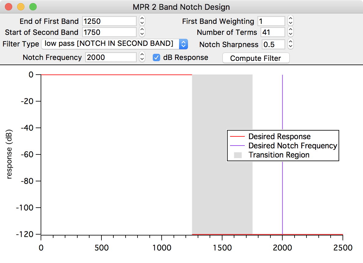
MPR 2 Band Notch Design Graph

The MPR 2 Band Notch design graph is identical to the MPR 2 Band design graph except you can place a transmission zero (or "notch") at a precise frequency.

The resultant filter is technically a cascade of two filters but the program combines (convolves) both coefficient arrays into a single filter. For a discussion of the technique used by this design, refer to page 86 of Elliot.

The parameters are:

• ‘End of First Band’ specifies the highest frequency in the frequency band beginning at 0 Hz (D.C.). In the example graph, the first band’s frequency range extends from 0 Hz to 0.25 Hz.

  If the filter type is "low pass", the first band is a passband, where the nominal filter gain is 1.0, or 0 dB.

  If the filter type is "high pass", the first band is a stopband, where the nominal filter gain is 0, or or -∞ dB

• ‘Start of Second Band’ specifies the lowest frequency in the second band. The second band ends at the Nyquist frequency (0.5 Hz in the example graph).

  If the filter type is "low pass", the second band is a stopband.

  If the filter type is "high pass", the second band is a passband.

  The frequencies between the end of the first band and the start of the second band (0.25 Hz to 0.35 Hz in the example) are called the "transition band", where the filter gain is changing from approximately 1.0 to approximately 0.0.

• ‘Filter Type’ chooses either a lowpass or a highpass design.

• ‘Notch Frequency’ specifies the center frequency of the transmission zero ("notch").

  Since the notch is always located in the stopband, if a low pass filter is chosen, the notch frequency must be in the second band. For a high pass filter, the notch must be in the first band.

• ‘First Band Weighting’ determines the relative accuracy in the first band compared to the second band. For example, if this number is greater than 1 then the error in the first band will be reduced at the expense of increased error in the second band.

• ‘Number of Terms’ specifies the number of coefficients in the FIR filter. This is also the number of values in the "coefs" filter wave.

  An odd number of coefficients is recommended, especially for high pass designs.

• ‘Notch Sharpness’ can be used to adjust the relative width of the notch. It does so by adjusting the relative gain of the two cascaded filter sections.

You may find that the notch will not work properly if the quantization is too coarse (if too few quantization bits are specified in the Set IFDL Parameters dialog).

MPR 3 Band Design Graph

The MPR 3 Band design graph can be used to design band pass and band reject filters using the McClellan-Parks-Rabiner equiripple technique.

The parameters are:

• ‘End of First Band’ specifies the highest frequency in the frequency band beginning at 0 Hz. In the example design graph, the first band’s frequency range extends from 0 Hz to 0.1 Hz.

  If the filter type is "band reject", the first band is a passband, where the nominal filter gain is 1.0, or 0 dB.

  If the filter type is "band pass", the first band is a stopband, where the nominal filter gain is 0, or or -∞ dB.

• ‘Start of Second Band’ specifies the lowest frequency in the second (middle) band.

  If the filter type is "band reject", the second band is a stopband; if "band pass", the second band is a passband.

  The frequencies between the end of a band, and the start of the next band are "transition bands", where the filter gain is changing from approximately 1.0 to approximately 0.0.

• ‘End of Second Band’ specifies the highest frequency in the second band.

• ‘Start of Third Band’ specifies the lowest frequency in the last band which ends at the Nyquist frequency (0.5 Hz in the example design graph).

  Like the first band, if the filter type is "band reject", the third band is a passband; if "band pass", it is a stopband.

• ‘Filter Type’ chooses either a band pass or band reject design.

• ‘Second Band Weighting’ determines the relative accuracy in the second (middle) band compared to the other bands. For example, if this number is greater than 1 then the errors in the second band will be reduced at the expense of increased errors in the second and third bands.

• ‘Number of Terms’ specifies the number of coefficients in the filter. This is also the number of values in the "coefs" filter wave.

  An odd number of coefficients is recommended, especially for band reject designs.

MPR Differentiator Design Graph

This design graph creates a differentiator filter using the McClellan-Parks-Rabiner equiripple method. The filter has a straight-line gain vs frequency response from 0 Hz to the ‘End of First Band’ value, with a slope equal to the given ‘Slope’ value:

The dialog parameters are:

• ‘End of First Band’ specifies the highest frequency in the frequency band beginning at 0 Hz. In the example design graph, the first band extends from 0 Hz to 450 Hz.

• ‘Slope’ determines the slope of the magnitude response. A value of 1, for example, causes the response to attempt to reach 0.5 at the Nyquist frequency. A slope of 2 attempts to reach a response of 1.0 at the Nyquist frequency, etc.

  The response at the ‘End of First Band’ is:

  Slope * End of First Band / Sampling Frequency

  For the example graph:

  1 * 450 Hz / 1000 Hz = 0.45

• ‘Number of Terms’ specifies the number of coefficients in the differentiator filter. This is also the number of points in the "coefs" filter wave.

The number of filter coefficients should be even and should be relatively small (if too large, IFDL will give a failure-to-converge error).

MPR Hilbert Design Graph

This design graph produces Hilbert transformers using the McClellan-Parks-Rabiner equiripple method. Such filters are used in the field of communications for modulation and demodulation for their unusual property of shifting all frequencies in the passband by -90 degrees.

Hilbert filters designed with a symmetrical passband have another unusual property of having half of the coefficients equal to zero (meaning that hardware implementations require half the number of multipliers):

The conditions required for these zero coefficients are:

1. Start of Pass Band = Nyquist Frequency - End of Pass Band

2. Number of Terms is an odd number.

If you leave the ‘Symmetrical’ checkbox checked, IFDL keeps the ‘Start of Pass Band’ and ‘End of Pass Band’ values adjusted to satisfy those conditions.

The Hilbert design graph is the only one that shows the phase of the computed filter (other filters have zero or completely linear phase shift). The phase trace and axis are drawn using red to help you associate the phase trace with its axis.

The parameters are:

• ‘Start of Pass Band’ specifies the lowest frequency in the passband. In the example dialog, the passband begins at 0.05 Hz.

• ‘End of Pass Band’ specifies the highest frequency in the pass band. In the example graph, the pass band ends at 0.45 Hz.

  The filter is usually specified with a passband centered about half the Nyquist frequency, or one quarter of the sampling frequency. If this isn’t the case, the stopbands may have unexpected characteristics, and every other coefficient will not be zero.

• ‘Symmetrical’ instructs IFDL to keep the passband centered around half the Nyquist frequency by adjusting ‘Start of Pass Band’ when you change ‘End of Pass Band’, or vice-versa.

• ‘Terms’ specifies the number of coefficients in the Hilbert transformer filter. This is also the number of points in the filter wave.

  The number of filter terms is always odd.

MPR Arbitrary Filter Design Graph

The Arbitrary Filter Design graph is a bit different than the other filter design graphs.

Using various means, you can completely specify:

• desired frequency response,
• weighting,
• transition regions,
• number of filter terms,

to the MPR equiripple algorithm. With this added power comes some complexity:

Desired Frequency Response

The main task is to create the desired response curve.

The Preset controls help you get started. It is based on the idea of "bands" of frequencies where the desired response (or gain) alternates between 0 and 1.0.

The example graph above shows the result of choosing 3 bands and clicking the "Preset Bands" button.

You can edit the response trace with the mouse.

Editing the Response and Weighting Traces

Clicking on the ‘Edit Response’ or ‘Edit Weighting’ buttons invokes the GraphWaveEdit mode on the corresponding trace. Here we’ve clicked on the ‘Edit Response’ button in the example graph:

Use the mouse to edit the trace to define the desired filter parameters with these methods:

To add a point to the response or weighting trace	Click anywhere on the trace where you want to add the point.
To edit a point already on the trace	Click and hold on the existing point and drag it to the new position.
To remove an existing point	Hold down the Alt key to get the lightning bolt cursor, and click the point.
To move a straight-line portion of the trace	Hold down the Ctrl key to get the 4-arrows cursor, click and hold on the line, and drag it to the new position.
	Hold down the shift key to constrain movement to vertical and horizontal displacements.

When you are done editing the trace, click the ‘Finish Response’ or ‘Finish Weighting’ button.

Weighting

The Preset bands button initially sets the weighting to be 1.0 where there are pass bands or reject bands, and to 0.0 in the transition bands. (This means that we don’t care what the response is in those regions.)

You can force the design algorithm to give higher priority to portions of the desired response by assigning a higher weighting value to that frequency range. The default weighting value is 1.0, the value applied to all frequencies when you click the ‘None’ weighting button.

There are two ways to assign weighting values:

• Click the ‘Edit Weighting’ button, and edit the weighting trace directly.

• Use the marquee to set a range to a constant value over the frequency range enclosed by the marquee.

To set the weighting using the marquee:

1. Sweep out a marquee over the frequency range you will assign a constant weighting value to.

2. Click inside the marquee and choose ‘Set_Weighting_Value’ from the marquee menu.

3. Enter the weighting value in the dialog that appears.

4. Click Continue.

Transition Regions

The transition regions indicate frequencies where we expect the response to change from a reject band to a pass band or vice versa, so we don’t want to constrain the response to a particular value.

Using transition regions allows the filter design algorithm more freedom to optimize the response in places where we do care about what the response is.

Editing Transition Regions

Transition regions are added and removed using the marquee menu.

To remove one or more transition regions:

1. Sweep out a marquee over the frequency range you will remove transition region(s) from.

2. Click inside the marquee and choose ‘Remove_Transition_Region’ from the marquee menu.

To add a transition regions, follow the same procedure, but choose ‘Add_Transition_Region’, instead.

You can extend a transition region by overlapping the marquee with an existing transition region and choosing ‘Add_Transition_Region’:

You can also trim a transition region by overlapping the marquee and choosing ‘Remove_Transition_Region’.

Filter Terms

An odd number of filter terms is required because it eliminates phase shift in the filtered result.

Increasing the number of terms reduces the errors in the actual filter response. ("Errors" in this context means deviations from the desired response trace.)

Increasing the number of terms also increases the number of ripples in the response.

Kaiser Maximally Flat Design Graph

This low pass design technique, due to Kaiser, has the sometimes very desirable property of producing FIR filters having absolutely no ripple within the limits of quantization. Naturally such filters have many more terms than an equivalent equiripple design. The number of coefficients are calculated based on the entered parameters.

The parameters are:

• ‘Transition Frequency’ is the 50% gain point of the response curve.

• ‘Transition Width’ is the width of the response curve from 95% gain to 5% gain.

Avoid specifying excessively narrow transition widths, or transition frequencies near the Nyquist frequency.

IFDL prevents you from entering obviously wrong values. Even so, some values may cause the FMaxflat operation to run for a long time while spinning the "beach ball" cursor.

If this happens, your best recourse may be to stop the operation by typing User Abort Key Combinations or pressing the Abort button.

Then try using a larger transition width or a lower transition frequency.

Kaiser Low Pass Design Graph

This low pass FIR filter design is based on the Kaiser window. It is principally provided for teaching purposes. See Window Filters Design Graph for an explanation.

The parameters are:

• ‘End of Pass Band’ is the highest frequency in the passband. The passband extends from 0 Hz to this frequency, where the nominal gain is 1, or 0 dB.

• ‘Start of Stop Band’ is the lowest frequency in the stopband. The stopband extends from this frequency to the Nyquist frequency, where the nominal gain is 0, or -∞ dB.

  The frequencies between the pass and s top bands define the transition band, where the gain is changing from 1 to 0.

• ‘Number of Terms’ chooses an even or odd number of terms. As with the Kaiser MaxFlat design, the number of coefficients are calculated based on the desired properties.

• ‘Min Stop Band Attenuation (dB)’ is a positive number expressing the maximum gain in the stop band in decibels.

Window Filters Design Graph

This low or high pass method is the classic "window" method of FIR filter design if the ‘End of First Band’ frequency is equal to ‘Start of Second Band’ (that is, if there is a zero-width transition region).

note

Igor 6 and later include window filter design independently of IFDL. Both the Igor 6 window filter design and the IFDL window filter design result in a set of FIR coefficients that can be analyzed for frequency response using the FFT and applied to data using the FilterFIR operation.

The parameters are:

• ‘End of First Band’ is the highest frequency in the first band.

  If the ‘Filter Type’ is "low pass", the first band is the pass band; if "high pass", it is the stopband.

• ‘Start of Second Band’ is the lowest frequency in the second band. The second band extends from this frequency to the Nyquist frequency.

  If the ‘Filter Type’ is "low pass", the second band is the stopband; if "high pass", it is the passband.

  The frequencies above the ‘End of First Band’, and below the ‘Start of Second Band’ are the transition region, where the gain is changing between 1 and 0.

• ‘Filter Type’ selects either a low pass or high pass filter.

• ‘Number of Terms’ specifies the number of coefficients in the FIR filter. This is the number of values in the "coefs" filter wave.

• ‘Window’ specifies the window function used on the coefs wave. The "Kaiser[1]" selection is the Kaiser window with ß = 1.

Window-based Filter Design Details

The Window Filter Design algorithm constructs a frequency-domain magnitude response step with the edges at the specified frequencies:

If a reasonable transition band width is specified then a smooth frequency domain transition between the bands is applied, rather than the classic abrupt edge. You can try different transition curves by editing the IFDLRoundedEdge function in the "Window Filters.ipf" procedure file.

The designed response is inverse-FFT’d to produce the impulse response:

It is then truncated to the entered value for ‘Number of Terms’ and multiplied by the selected ‘Window’ function:

Given the availability of the McCellan-Parks-Rabiner method, this technique is mostly for instructional value since it uses more filter terms to achieve the same performance.

IIR Analog Prototype Design Graph

The IIR Analog Prototype design graph was added to IFDL in version 4. It designs Infinite Impulse Response filters whose response mimics that of traditional analog electronic Butterworth, Chebyshev, and Bessel filters.

note

Igor 6 and later include IIR filter design independently of IFDL using the Filter Design and Application Dialog. Those IIR filters use only Butterworth designs.

The main functions of this design graph specify:

• filter type (highpass, lowpass, bandpass, bandstop, or notch-only),
• band edge(s),
• filter order,
• analog prototype (Bessel, Butterworth, or Chebyshev),
• additional notches.
• implementation (Direct Form I or Cascade DF II),

For reference or for comparison to other filter design programs, the design graph provides for display of:

• poles and zeros in the Z-plane
• coefficient values in a table,
• for cascade implementations, the frequency response of each section.

Filter Type

You can choose from the basic two-band filter choices and an additional "notch only" option.

When "notch only" is selected, no band edges apply: only the notch settings. See the Additional Notches section below.

Band Edges

Depending on which filter type is chosen, 1^st Band and 2^nd Band define the approximate –3 dB corner frequencies of the filter. In the analog filter world, these correspond to the "poles" of the filter. For bandpass and bandstop filter types, the value of 1^st Band must be less than or equal to the value of 2^nd Band.

Filter order

"Filter order" refers to the number of poles (and also the number of zeros) in the filter. Higher order filtering has a steeper transition region:

A filter of order 2 (a "second order filter") has two poles and two zeros. This is also called a "bi-quad" or "bi-quadratic" filter. The second order filter is the basic building block (or "section") of the Cascade Direct Form II implementation. See the "Implementation" section below.

Analog Prototype

The IIR filters are designed by transforming classical analog filter designs from the Laplace (or "S-plane") into the Z-transform plane (or "Z-plane") using a bilinear transformation.

Analog filters are designed by computing the position of "poles" and "zeros" in the complex S plane. These poles correspond to infinite maxima and the zeros to, well, zeros, in the Laplace transform of the filter transfer function H(s):

$$\displaystyle H(s)=K \bullet\left(\frac{\left(s-z_{1}\right) \cdot\left(s-z_{2}\right) \ldots}{\left(s-p_{1}\right) \cdot\left(s-p_{2}\right) \ldots}\right)$$

where p₁, p₂, etc are the pole locations in the complex (Laplace) S plane s = α+ jω. The ω part in jω is the pole frequency (in radians/second) in the S plane. ω can have any value from -∞ to +∞.

The Butterworth, Bessel, and Chebyshev analog filters are designed to have poles in different locations in the S-plane, which result in different frequency responses:

• Bessel filters tend to have the most linear phase response of the three choices.

• Butterworth filters have a very smooth passband with a sharper cutoff shape than the Bessel filter.

• Chebyshev filters exhibit a still-sharper cutoff at the expense of introducing ripple in the passband.

Here are the pole locations for second order low pass filters with 2nd Band set to ½ of the Nyquist frequency:

These second order filter example also have zeros at s = 0 + j ∞ and s = 0 – j ∞, which aren’t shown.

The S plane designs are all frequency-normalized lowpass filters. The S plane design frequencies are computed in Hz by dividing the 1st and/or 2nd band frequencies by the sampling frequency, and then adjusted so that when the poles are mapped into the Z plane the desired cutoff frequency is obtained.

The S plane poles and zeros are then frequency scaled to account for the sampling frequency, converted to highpass, bandpass, or bandstop, and then converted into the Z plane for digital filter realization.

Here are the corresponding Z plane poles of the filters shown above (the sampling frequency has been set to 1 Hz):

Digital filters are designed in the Z transform plane, which has a finite frequency range of 0 to the Nyquist frequency. The Z transform is beyond the scope of this Help, but basically it is a digital equivalent of the analog S or Laplace transform.

The conversion from S plane to Z plane is accomplished through the "bilinear transform" which maps an S plane value s = α + jω into the Z plane z = by the relation:

$$\displaystyle z=\frac{2+s}{2-s}$$

This relation maps s = 0 + j∞ to z = -1 + j0, (or z = e^jπ) so that the infinite frequency range ω= 0 + j0…∞ in the S plane is mapped to e^j0… e^jπ in the Z plane. This compresses the complete frequency response of the analog filter nonlinearly into the range from 0 to the Nyquist frequency:

These transformed poles and zeros (p'₁, p'₂, etc) form the corresponding Z transform filter transfer function H(z):

$$\displaystyle H(z)=K \bullet\left(\frac{\left(z-z_{1}^{\prime}\right) \cdot\left(z-z_{2}^{\prime}\right) \ldots}{\left(z-p_{1}^{\prime}\right) \cdot\left(z-p_{2}^{\prime}\right) \ldots}\right)$$

The realization of this function varies depending on the implementation (see "IIR Implementations", below).

Additional Notches

After the Z plane poles and zeros of the filter have been computed, one or more notches (aka "zeros") can be added to these filters.

Each zero is positioned on the unit circle of the Z plane at the angle corresponding to the zero’s frequency, where π corresponds to the Nyquist frequency.

Each zero has a corresponding pole placed near it whose placement affects the sharpness of the notch. The pole placement is computed based on the notch "Q", as shown above.

IIR Implementations

Once the Z plane poles and zeros have been computed, the filter design is actually implemented using either a Direct Form I or Cascaded Bi-Quad Direct Form II implementation.

Each implementation method creates a different kind of IIRCoefs filter wave.

Direct Form I

See Quick Review of Digital Filter Design for a diagram of the Direct Form I filter. An IIR filter’s transfer function in pole-zero form is:

$$\displaystyle H(z)=K \prod_{k=1}^{N} \frac{z-z_{k}^{\prime}}{z-p_{k}^{\prime}}$$

To implement the Direct Form I filter, the products are each expanded into an Nth order polynomial in z^-1:

$$\displaystyle H(z)=\frac{Y(z)}{X(z)}=\frac{a_{0}+a_{1} z^{-1}+a_{2} z^{-2} \ldots+a_{N} z^{-N}}{b_{0}+b_{1} z^{-1}+b_{2} z^{-2} \ldots+b_{N} z^{-N}}$$

Where Y(z) is the Z transform of the output signal and X(z) is the Z transform of the input signal. Cross-multiplying X(z) and the right-hand-side denominator yields:

$$\displaystyle \mathrm{Y}(z)\left(b_{0}+b_{1} z^{-1}+b_{2} z^{-2} \ldots+b_{N} z^{-N}\right)=X(z)\left(a_{0}+a_{1} z^{-1}+a_{2} z^{-2} \ldots+a_{N} z^{-N}\right)$$

The equivalent time-domain "finite difference equation" is computed by substituting x[i-n] for X(z)z^-n (an inverse Z transformation) – and similarly for y and Y(z) – and then solving for the digital time-domain output signal y[i]:

$$\displaystyle y[i]=\frac{1}{b_{0}}\left\{a_{0} x[i]+a_{1} x[i-1] \ldots+a_{N} x[i-N]-b_{1} y[i-1] \ldots+b_{N} y[i-N]\right\}$$

The IFDL implementation of this filter is a real-valued two-column wave with the numerator coefficients a₀ through a_N in the first column, and the denominator coefficients b₀ through b_N in the second column:

		Numerators	Denominators
	Row	Column 0	Column 1
	0	a0	b0
	1	a1	b1
	…	…	…
	N	aN	bN

Cascaded Bi-Quad Direct Form II

See Quick Review of Digital Filter Design for a diagram of the cascade filter.

Each bi-quad section of the cascade applies second order filtering (two poles and two zeros) before passing the result to the next section, each in turn, until all the designed poles and zeros have been applied. This implementation divides the Z plane filter transfer function into groups of products. For example a 4th order filter:

$$\displaystyle H(z)=K \bullet \frac{\left(z-z_{1}^{\prime}\right)\left(z-z_{2}^{\prime}\right)\left(z-z_{3}^{\prime}\right)\left(z-z_{4}^{\prime}\right)}{\left(z-p_{1}^{\prime}\right)\left(z-p_{2}^{\prime}\right)\left(z-p_{3}^{\prime}\right)\left(z-p_{4}^{\prime}\right)}$$

is divided into two sections of 2nd order filters:

$$\begin{array}{l} \displaystyle H_{1}(z)=K_{1} \cdot \frac{\left(z-z_{1}^{\prime}\right)\left(z-z_{2}^{\prime}\right)}{\left(z-p_{1}^{\prime}\right)\left(z-p_{2}^{\prime}\right)} \\ \\ \displaystyle H_{2}(z)=K_{2} \cdot \frac{\left(z-z_{3}^{\prime}\right)\left(z-z_{4}^{\prime}\right)}{\left(z-p_{3}^{\prime}\right)\left(z-p_{4}^{\prime}\right)} \end{array}$$

and the combined result H₁(z)H₂(z) = H(z).

Each section’s transfer function is multiplied out into a polynomial in powers of z^-1. For example, H₁(z) becomes:

$$\displaystyle H_{1}(z)=\frac{a_{0}+a_{1} z^{-1}+a_{2} z^{-2}}{b_{0}+b_{1} z^{-1}+b_{2} z^{-2}}$$

This second order ratio is then transformed into the equivalent "finite difference" form:

$$\displaystyle y[i]=\frac{1}{b_{0}}\left\{a_{0} x[i]+a_{1} x[i-1]+a_{2} x[i-2]-b_{1} y[i-1]+b_{2} y[i-2]\right\}$$

The IFDL implementation of this filter is a real-valued six-column wave whose every row corresponds to one of the bi-quad sections. Within each row, the first three columns contain the numerator coefficients a₀, a₁, and a₂, and the next three columns contain the denominator coefficients b₀, b₁, and b₂:

Options for Cascaded Bi-Quad Direct Form II

The poles and zeros are grouped into a section based on several criteria:

• The poles closest to (or, optionally, farthest from) the unit circle are assigned to the first section, taking care to keep conjugate pairs together in the same section.

• Zeroes closest to those poles are placed into the same section, also taking care to group conjugate pairs (if any) in the same section.

• If the number of poles (and zeros) is odd, a pole and zero at z=(0,0) is used to fill out the last section (each section requires two poles and two zeros).

The default grouping option puts poles closest to the unit circle in the first section, as shown in this example of pole/zero grouping for a three-section filter implementing a 4^th order filter with one additional notch:

The grouping criteria can be reversed in the "Section Gains, Options" graph by checking the ‘Reverse Pole and Zero Grouping’ checkbox.

In the H₁(z) and H₂(z) formulas, note that the apportionment of K into K₁ and K₂ can be done many ways. The values IFDL uses for K₁ and K₂, etc can be modified in the "Section Gains, Options" graph, too.

The default method sets K₂…K_n to 1 and then calculates a K₁ so that the overall frequency response’s maximum gain is 1.0.

Selecting ‘Normalize Each Section’ applies this calculation to each section’s frequency response. This is desirable when the sections are implemented with fixed-point arithmetic (e.g., in hardware) to prevent numerical overflow. The drawback is that by normalizing each section’s maximum gain to 1.0 the overall maximum gain can be almost any value! In hardware systems, this can be overlooked when an amplifier, multiplier, or attenuator can be used to restore the overall gain.

Selecting ‘Except the First Section’ restores the overall frequency responses’s maximum overall gain to 1.0 while normalizing the remaining sections.

Advantages of Cascaded Bi-Quad Direct Form II

The Cascaded Bi-Quad Direct Form II implementation works better than the Direct Form I when the filter order approaches 10 because it avoids computing differences of numbers with wildly different magnitudes. (A 10^th order IIR filter uses 22 terms.)

Cascaded Bi-Quad Direct Form II also works better when limited-precision (say, 32-bit) hardware is used. It is a popular design for audio and video processing using 32-bit integer arithmetic.

However, because of the cascading, the overall delay is higher than the Direct Form I.

Plot Poles and Zeros

Clicking the ‘Plot Poles and Zeros’ button displays the filter’s poles and zeros in a polar graph of the Z plane (See "IIR Implementation", above, for examples.)

Poles are shown as X’s, and zeros as O’s. Often a filter has multiple zeros at z=-1+j0 or z=1+j0. These are drawn as concentric O’s of increasing size. The first 10 zeros at a location are drawn this way: additional zeros are all drawn at the maximum size.

When the Cascade implementation is chosen, the poles and zeros are drawn with colors that indicate the section grouping.

Show Coefficients

Clicking the ‘Show Coefficients’ button displays the IIRCoefs wave in a table that is formatted to explain the coefficients.

For a Direct Form I implementation, IIRCoefs is implemented as a two-column waveform with dimension labels showing the tap delay ("z^-3" means the tap delay of 3 samples) and whether the coefficient is a numerator or denominator in the Direct Form I H(z) formula:

For a Cascade DF II implementation, IIRCoefs is implemented as a six-column waveform with dimension labels showing the section number and the the coefficient in the Direct Form II H(z) formula:

IFDL Operations

IFDL relies on the FMaxFlat and Remez operations to compute FIR filter coefficients.

These operations are built into Igor 8 and later (with some additional features) and were provided by the IFDL XOP for earlier versions of Igor.

You normally won’t need to write code that uses these operations.

See Also

FilterFIR, FilterIIR

IFDL Bibliography

IFDL was created using the following resources:

[Elliot]

Elliot, Douglas F., contributing editor, Handbook of Digital Signal Processing Engineering Applications, Academic Press, San Diego, CA, 1987.

[Embree]

Embree, Paul M, Kimble, Bruce, C Language Algorithms for Digital Signal Processing, Prentice Hall, Englewood Cliffs, New Jersey 07632, 1991.

[IEEE]

IEEE Digital Signal Processing Committee, Editor, Programs for Digital Signal Processing, IEEE Press, New York, 1979

[Kaiser]

Kaiser, J.F., Design subroutine (MXFLAT) for symmetric FIR low pass digital filters with maximally flat pass and stop bands. in [IEEE].

[Lynn]

Lynn, Paul A., Fuerst, Wolfgang, Introductory Digital Signal Processing with Computer Applications., Second Edition, John Wiley & Sons, Ltd., 1998.

[McClellan]

J. H. McClellan, T.W. Parks, and L. R. Rabiner, A computer program for designing optimum FIR linear phase digital filters. IEEE Transactions on Audio and Electroacoustics, AU-21, 506-526 (December 1973).

[Press]

Press, William H., Numerical recipes in C: The art of Scientific Computing, Cambridge University Press, 1988

[Rabiner]

L. R. Rabiner, J. H. McClellan, and T.W. Parks, FIR digital filter design techniques using weighted Chebyschev approximation, Proc. IEEE 63, 595-610 (April 1975)

[Ramirez]

Ramirez, Robert W., The FFT: Fundamentals and Concepts, Tektronix, 1975. Part Number 070-1754-00.

IFDL Troubleshooting

When Things Go Wrong

"If anything can go wrong, it will."

— Edsel Murphy

Here are the problems you are most likely to encounter with IFDL, and our suggested solutions. Each section heading is one of:

• text that appears in a warning dialog

• text that is printed to the history window

• a description of a problem

Each section describes the likely causes of the problem and proposes solutions.

Problems are listed roughly in the order you might encounter them while using IFDL.

Macro Scan Error - include file not found

You can add the IFDL or IFDL Apply Filter procedures to an experiment by typing:

#include ":IFDL v4 Procedures:IFDL"

or:

#include ":IFDL v4 Procedures:IFDL Apply Filter"

in any procedure window, and clicking the Compile button at the bottom of the procedure window.

Normally the compile button will disappear without producing any error dialog. However, if you see the Procedure Scan Error dialog:

there are three likely causes:

• The #include statement has a typographical error, possibly a missing ":" or space character,

• The #include statement is referring to an old IFDL version (no "v4" in the path),

• The IFDL v4 Procedures folder is missing from your Igor Pro Folder. Reinstalling Igor 8 will correct this.

Igor Changes a Value I Entered in a Control

IFDL will prevent you from entering an illegal value based on the current settings.

There are two common scenarios:

• you are typing an even value into a ‘Number of Terms’ control

• you are typing a frequency value into a control such as ‘End of First Band’

Many of the filter designs require an odd value for ‘Number of Terms’. This avoids introducing a time delay of ½ the sampling interval in the filtered output. For example, typing "18" into the Hilbert design graph’s ‘Terms’ control, will provoke IFDL into setting the value to 19, the next legal value.

Similarly, the frequency values are checked against the other frequency values and are "clipped" to "legal" values. Changing the ‘End of First Band’ frequency value in the MPR 2 Band Notch design graph shown below to a value exceeding 0.35 would result in a negative width transition band:

IFDL will change the value you entered to leave at least a zero-width transition band.

For this same reason, the maximum and minimum values for the SetVariable controls prevent you from specifying improper values using the up and down arrows. These limits are automatically updated when, for example, you change the value of ‘Start of Second Band’.

Design something, first!

Couldn’t find "coefs" wave in current data folder!

If you see one of these dialogs:

<img src="MD_images/Igor Filter Design Laboratory/CouldntFindCoefs.png"coefs"_wav_0.png" width="75%"/>

then IFDL looked for the "coefs" FIR filter wave in the current data folder and didn’t find it (this can also happen when IFDL is looking for the "IIRCoefs" IIR filter wave).

These dialogs appear if you haven’t clicked any ‘Compute Filter’ button before choosing ‘Normalize Design Coefficients...’, ‘Design Report Layout’, or ‘Save Design’ from the IFDL menu, or if the current data folder has been changed from the data folder used when filters were computed.

You should either:

• click one of the filter design buttons in the IFDL control panel,

• design a filter,

• and click ‘Compute Filter’

or:

• Use the Data Browser (in the Data menu) to reset the current data folder to the data folder used when the filter designs were computed.

and try again.

(Normalize Design Coefficients gives this error when it can’t find the "preQuantCoefs" wave in the WM_IFDL data folder. PreQuantCoefs is created when you click the ‘Compute Filter’ button, too.)

See also "Coefs Wave isn’t being updated" in the next section for more about the "coefs" and "IIRCoefs" waves and IFDL’s use of data folders.

Current Data Folder is wrong

Coefs Wave isn’t being updated

IFDL creates many waves, variables, and strings in the root:Packages:WM_IFDL data folder. However, it stores and updates the coefs and IIRCoefs waves along with various filter results in the "current data folder".

It is possible for IFDL to lose track of the current data folder after some other error has occurred, and so IFDL might have created another coefs wave in what IFDL thinks is your intended current data folder.

If there is any doubt about the value of the current data folder, choose Data Browser from the Data menu to display the Data Browser:

If the current data folder has been changed, you should:

• Delete any "coefs" wave in the WM_IFDL data folder (or wherever the bogus coefs wave has ended up).

• Reset the current data folder to your preferred value.

  For most users, this will be the root: data folder. In this example, drag the red arrow from WM_IFDL up to root: or enter this command in Igor’s command line:

  SetDataFolder root:

The filter design did not converge ...

Failure to converge after n iterations

If the design requirements are too strict — an unreasonably small transition region between the passband and stopband, a maximum error which is too small, or too many filter terms — then the MPR algorithm may fail to converge, resulting in an error dialog:

Click ‘OK’ and change the design parameters to avoid the problem. The problem is often caused by specifying too many filter coefficients.

This dialog appears only if the filter design fails to converge after 1, 2, or 3 iterations. If more iterations occurred before the convergence failed, the dialog isn’t shown (because the filter has a reasonable chance of being okay).

IFDL always places a "failure to converge after n iterations" error message in the command window’s history area warning you that the filter may produce undesirable results.

note

Coefficients are not quantized.

This informational message appears in the history window when you select ‘Normalize Design Coefficients...’ in the IFDL menu, and the ‘quantize the coefficients" popup is set to "No":

‘No’ instructs IFDL to ignore the ‘bits of quantization’ setting in the SetIFDLParameters dialog during the normalization:

See Setting the IFDL Parameters for more about ‘bits of quantization’.

warning

data samp freq = XX Hz (sample freq = YY Hz)

When you invoke the ‘Apply Filter’ item from the IFDL menu:

and choose ‘warn if not correct’ for the ‘data wave sample frequency’ setting, you may see this warning dialog:

This dialog means three things:

1. There is a mismatch between the data’s sampling frequency (5000 Hz in this example), and the IFDL design sampling frequency (1 Hz in this example).

2. The sampling frequencies of data wave and the filter wave were not changed.

3. The filtered result is as if the filter’s frequency range was scaled to match the data’s frequency range.

No dialog is shown when you choose the ‘force to samp freq’ setting for the popup.

In that case, IFDL will scale the data wave’s frequencies to the filter’s frequencies.

See the next section for an explanation of "Filter Frequency Scaling".

Filter sampling frequency doesn’t match data

warning

Filter sampling frequency does not match data

After adding:

#include ":IFDL v4 Procedures:IFDL Apply Filter"

to your procedure window, you can invoke the ApplyFilterToData macro from the Analysis Menu:

If you choose a filter coefficient wave whose sampling frequency does not match the data wave, you will see a dialog like this:

Choosing "Yes" will scale the filter’s sampling frequency to match the data’s sampling frequency, and Igor will print a message like this one in its history window:

Filter Frequency Scaling

The filter scaling is most easily visualized in the frequency domain. Here is an example kaiserMaxFlat filter’s frequency response designed with a 10 Hz sampling frequency:

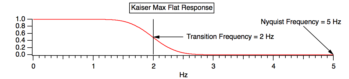
The filter rejects frequencies above 2 Hz, and is designed for data sampled at 10 Hz (the Nyquist frequency is ½ the sample rate).

The data in this example, however, is sampled at 1 Hz, and the maximum frequency content (the Nyquist frequency) is 0.5 Hz:

When Igor applies the 10 Hz filter to the 1 Hz data, the result is as if the filter’s frequency axis had been scaled to match the data’s frequency range:

The scaled filter rejects frequencies above 0.2 Hz, a factor of 10 lower than the original design.

IIR Cutoff Frequency isn’t what you specified.

Adding notches near the cutoff frequency (band edge) distorts the frequency response. You can move the notch farther from the band edge, or sharpen the notch by increasing Q to lessen the effect the notch has on the cutoff frequency, or you can compensate by altering the requested cutoff frequency.

The Chebyshev cutoff frequency is affected by the specified amount of passband ripple: less ripple pushes the cutoff frequency out. You can compensate by altering the requested cutoff frequency.

IIR Notches aren’t very deep.

The frequency resolution used to compute the response may need to be increased to accurately gauge the notch response. Choose a higher value for ‘Frequency Resolution’ in the ‘Set IFDL Parameters…’ dialog. See Setting the IFDL Parameters.

Switch to Cascade DF II implementation.

Related Topics

Digital Filtering, Smoothing, Convolution.