Image Processing
Image processing is a broad term describing most operations that you can apply to image data which may be in the form of a 2D, 3D or 4D waves. Image processing may sometimes provide the appropriate analysis tools even if the data have nothing to do with imaging. Under Image Plots we described operations relating to the display of images. Here we concentrate on transformations, analysis operations and special utility tools that are available for working with images
You can use the IP Tutorial experiment (inside the Learning Aids folder in your Igor Pro folder) in parallel with this section. The experiment contains, in addition to some introductory material, the sample images and most of the commands that appear in this help file. To execute the commands, you can select them in this help file and type Ctrl-Enter.
Open the Image Processing Tutorial experiment
Image Transforms
The two basic classes of image transforms are color transforms and grayscale/value transforms. Color transforms involve conversion of color information from one color space to another, conversions from color images to grayscale, and representing grayscale images with false color. Grayscale/value transforms include, for example, pixel level mapping, mathematical and morphological operations.
Color Transforms
There are many standard file formats for color images. When a color image is stored as a 2D wave, it has an associated or implied colormap, and the RGB value of every pixel is obtained by mapping values in the 2D wave into the colormap.
When the image is a 3D wave, each image plane corresponds to an individual red, green, and blue color component. If the wave is of type unsigned byte (/B/U), values in each plane are in the range [0,255]. If the waves are not of type unsigned byte, the range of values is [0,65535].
There are two other types of 3D image waves. The first consists of 4 layers corresponding to RGBA where the 'A' represents the alpha (transparency) channel. The second contains more than three planes in which case the planes are grayscale images that can be displayed using the command:
ModifyImage imageName, plane=n
Multiple color images can be stored in a single 4D wave where each chunk corresponds to a separate RGB image.
You can find most of the tools for converting between different types of images in the ImageTransform operation. For example, you can convert a 2D image wave that has a colormap to a 3D RGB image wave. Here we create a 3-layer 3D wave named M_RGBOut from the 2D image named 'Red Rock' using RGB values from the colormap wave named 'Red RockCMap':
ImageTransform /C='Red RockCMap' cmap2rgb 'Red Rock'
NewImage M_RGBOut	// Resulting 3D wave is M_RGBOut
The images in the IP Tutorial experiment are not stored in the root datafolder, so many of the commands in the tutorial experiment include data folder paths. Here the data folder paths have been removed for easier reading. If you want to execute the commands you see here, use the commands in the "IP Tutorial Help" window. See the Data Folders for more information about data folders.
In many situations it is necessary to dispose of color information and convert the image into grayscale. This usually happens when the original color image is to be processed or analyzed using grayscale operations. Here is an example using the RGB image which we have just generated:
ImageTransform rgb2gray M_RGBOut
NewImage M_RGB2Gray	// Display the grayscale image
The conversion to gray is based on the YIQ standard where the gray output wave corresponds to the Y channel:
gray = 0.299 * red + 0.587 * green + 0.114 * blue.
If you wish to use a different set of transformation constants say {ci}, you can perform the conversion on the command line:
gray2DWave = c1 * image[p][q][0] + c2 * image[p][q][1] + c3 * image[p][q][2]
For large images this operation may be slow. A more efficient approach is:
Make/O/N=3 scaleWave={c1,c2,c3}
ImageTransform/D=scaleWave scalePlanes image	// Creates M_ScaledPlanes
ImageTransform sumPlanes M_ScaledPlanes
In some applications it is desirable to extract information from the color of regions in the image. We therefore convert the image from RGB to the HSL color space and then perform operations on the first plane (hue) of the resulting 3D wave. In the following example we convert the RGB image wave peppers into HSL, extract the hue plane and produce a binary image in which the red hues are nonzero.
ImageTransform /U rgb2hsl peppers	// Note the /U for unsigned short result
MatrixOp/O RedPlane=greater(5000,M_RGB2HSL[][][0])+greater(M_RGB2HSL[][][0],60000)
NewImage RedPlane			// Here white corresponds to red hues in the source
As you can see, the resulting image is binary, with white pixels corresponding to regions where the original image was predominantly red. The binary image can be used to discriminate between red and other hue regions. The second command line above converts hue values that range from 0 to 65535 to 1 if the color is in the "reddish" range, or 0 if it is outside that range. The selection of values below 5000 is due to the fact that red hues appear on both sides of 0° (or 360°) of the hue circle.
Hue based image segmentation is also supported through the operation ImageTransform using the keyword hslSegment. The same operation also supports color space conversions from RGB to CIE XYZ (D65 based) and from XYZ to RGB. See Handling Color and HSL Segmentation for further discussion.
Grayscale or Value Transforms
This class of transforms applies only to 2D waves or to individual layers of higher dimensional waves. They are called "grayscale" because 2D waves by themselves do not contain color information. We divide grayscale transforms into level mappings and mathematical operations.
Explicit Lookup Tables
Here is an example of using an explicit lookup table (LUT) to create the negative of an image the hard way:
Make/B/U/O/N=256 negativeLookup=255-x           // Create the lookup table
Duplicate/O baboon negativeBaboon
negativeBaboon=negativeLookup[negativeBaboon]   // The lookup transformation
NewImage baboon
NewImage negativeBaboon


In this example the negativeBaboon image is a derived wave displayed with standard linear LUT. You can also obtain the same result using the original baboon image but displaying it with a negative LUT:
NewImage baboon
Make/N=256 negativeLookup=1-x/255	 	// Negative slope LUT from 1 to 0
ModifyImage baboon lookup=negativeLookup
If you are willing to modify the original data you can execute:
ImageTransform invert baboon
Histogram Equalization
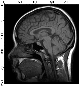
Histogram equalization maps the values of a grayscale image so that the resulting values utilize the entire available range of intensities:
NewImage MRI
ImageHistModification MRI
NewImage M_ImageHistEq
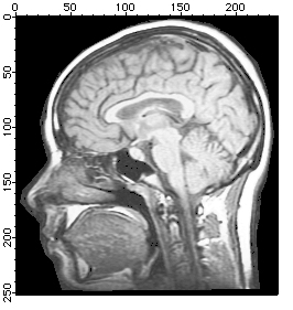
Adaptive Histogram Equalization
The ImageHistModification operation calculates a lookup table based on the cumulative histogram of the whole source image. The lookup table is then applied the output image. In cases where there are significant spatial variations in the histogram, a more local approach may be needed, i.e., perform the histogram equalization independently for different parts of the image and then combine the regional results by matching them across region boundaries. This is commonly referred to as "Adaptive Histogram Equalization".
ImageHistModification MRI
Duplicate/O M_ImageHistEq, globalHist
NewImage globalHist
ImageTransform/N={2,7} padImage MRI		// To make the image divisible
ImageHistModification/A/C=10/H=2/V=2 M_paddedImage
NewImage M_ImageHistEq
As you can see, we padded the image so that the numbers of pixels in the horizontal and vertical directions are divisible by the numbers of desired intervals. If you do not find the resulting adaptive histogram sufficiently different from the global histogram equalization, you can increase the number of vertical and horizontal regions that are processed:
ImageHistModification/A/C=100/H=20/V=20 M_paddedImage
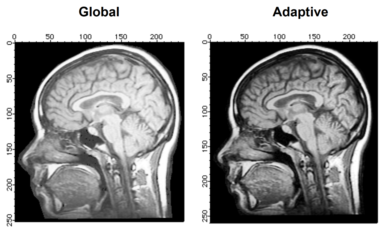
You can now compare the global and adaptive histogram results. Note that the adaptive histogram performed better (increased contrast) over most of the image. The increase in the clipping value (/C flag) gave rise to a minor artifact around the boundary of the head.
Threshold
The threshold operation is an important member of the level mapping class. It converts a grayscale image into a binary image. A binary image in Igor is usually stored as a wave of type unsigned byte. While this may appear to be wasteful, it has advantages in terms of both speed and in allowing you to use some bits of each byte for other purposes (e.g., bits can be turned on or off for binary masking). The threshold operation, in addition to producing the binary thresholded image, can also provide a correlation value which is a measure of the threshold quality
You can use the ImageThreshold operation either by providing a specific threshold value or by allowing the operation to determine the threshold value for you. There are various methods for automatic threshold determination:
| Iterated: | Iteration over threshold levels to maximize correlation with the original image | |
| Bimodal: | Attempts to fit a bimodal distribution to the image histogram. The threshold level is chosen between the two modal peaks. | |
| Adaptive: | Calculates a threshold for every pixel based on the last 8 pixels on the same scan line. It usually gives rise to drag lines in the direction of the scan lines. You can compensate for this artifact as we show in an example below. | |
| Fuzzy Entropy: | Considers the image as a fuzzy sets of background and object pixels where every pixel may belong to a set with some probability. The algorithm obtains a threshold value by minimizing the fuzziness which is calculated using Shannon's Entropy function. | |
| Fuzzy Means: | Minimizes a fuzziness measure that is based on the product of the probability that the pixel belongs in the object and the probability that the pixel belongs to the background. | |
| Histogram Clusters: | Determines an ideal threshold by histograming the data and representing the image as a set of clusters that is iteratively reduced until there are two clusters left. The threshold value is then set to the highest level of the lower cluster. This method is based on a paper by A.Z. Arifin and A. Asano (see reference below) but modified for handling images with relatively flat histograms. If the image histogram results in less than two clusters, it is impossible to determine a threshold using this method and the threshold value is set to NaN. Added in Igor Pro 7.00. | |
| Variance: | Determines the ideal threshold value by maximizing the total variance between the "object" and "background". See: | |
| http://en.wikipedia.org/wiki/Otsu's_method. | ||
| Added in Igor Pro 7.00. | ||
Each one of the automatic thresholding methods has its advantages and disadvantages. It is useful sometimes to try all different methods before you decide which method applies best to a particular class of images. The following example illustrates the different thresholding methods for the blobs image.
Comparison of Built-In Threshold Methods
This section shows results using various methods for automatic threshold determination.
The commands shown were executed in the demo experiment that you can open by choosing File->Example Experiments->Tutorials->Image Processing Tutorial.
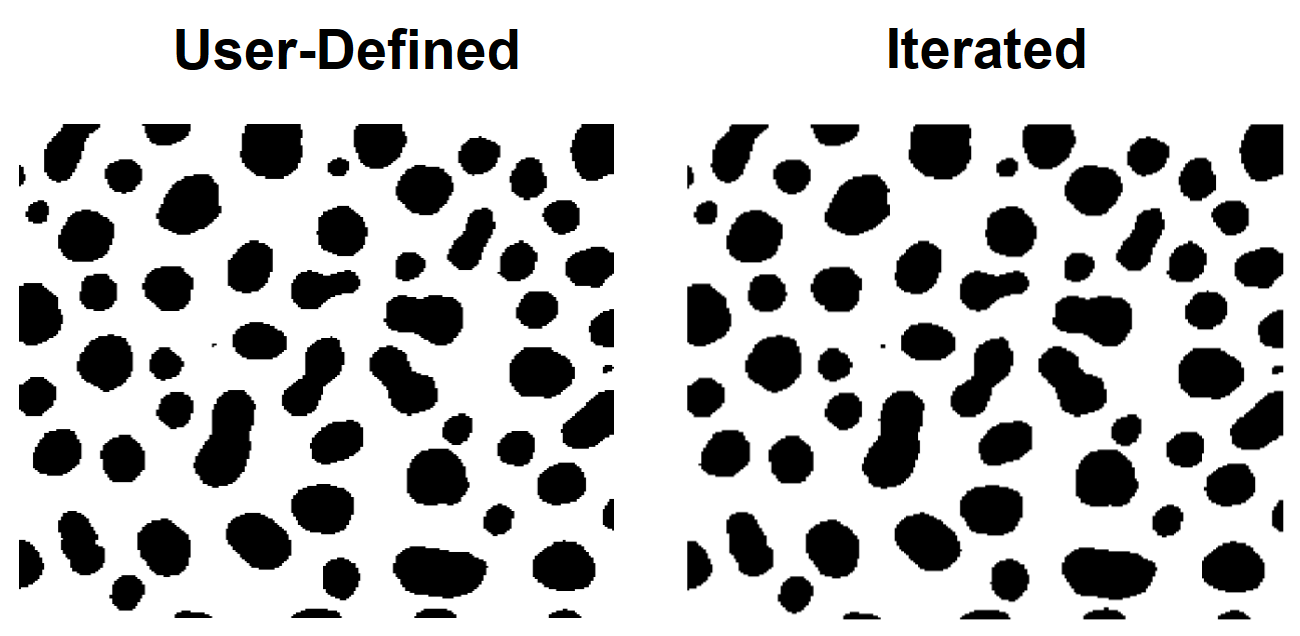
// User defined method
ImageThreshold/Q/T=128 root:images:blobs
Duplicate/O M_ImageThresh UserDefined
NewImage/S=0 UserDefined; DoWindow/T kwTopWin, "User-Defined Thresholding"

// Iterated method
ImageThreshold/Q/M=1 root:images:blobs
Duplicate/O M_ImageThresh iterated
NewImage/S=0 iterated; DoWindow/T kwTopWin, "Iterated Thresholding"
// Bimodal method
ImageThreshold/Q/M=2 root:images:blobs
Duplicate/O M_ImageThresh bimodal
NewImage/S=0 bimodal; DoWindow/T kwTopWin, "Bimodal Thresholding"

// Adaptive method
ImageThreshold/Q/I/M=3 root:images:blobs
Duplicate/O M_ImageThresh adaptive
NewImage/S=0 adaptive; DoWindow/T kwTopWin, "Adaptive Thresholding"

// Fuzzy-entropy method
ImageThreshold/Q/M=4 root:images:blobs
Duplicate/O M_ImageThresh fuzzyE
NewImage/S=0 fuzzyE; DoWindow/T kwTopWin, "Fuzzy Entropy Thresholding"

// Fuzzy-M method
ImageThreshold/Q/M=5 root:images:blobs
Duplicate/O M_ImageThresh fuzzyM
NewImage/S=0 fuzzyM; DoWindow/T kwTopWin, "Fuzzy Means Thresholding"

// Arifin and Asano method
ImageThreshold/Q/M=6 root:images:blobs
Duplicate/O M_ImageThresh A_and_A
NewImage/S=0 A_and_A; DoWindow/T kwTopWin, "Arifin and Asano Thresholding"

// Otsu method
ImageThreshold/Q/M=7 root:images:blobs
Duplicate/O M_ImageThresh otsu
NewImage/S=0 otsu; DoWindow/T kwTopWin, "Otsu Thresholding"

In the these examples, you can add the /C flag to each ImageThreshold command and remove the /Q flag to get some feedback about the quality of the threshold; the correlation coefficient will be printed to the history.
It is easy to determine visually that, for this data, the adaptive and the bimodal algorithms performed rather poorly.
You can improve the results of the adaptive algorithm by running the adaptive threshold also on the transpose of the image, so that the operation becomes column based, and then combining the two outputs with a binary AND.
Spatial Transforms
Spatial transforms describe a class of operations which change the position of the data within the wave. These include the operations ImageTransform operation with multiple keywords, MatrixTranspose, ImageRotate, ImageInterpolate, and ImageRegistration.
Rotating Images
You can rotate images using the ImageRotate operation. There are two issues that are worth noting in connection with image rotations where the rotation angle is not a multiple of 90 degrees. First, the image size is always increased to accommodate all source pixels in the rotated image (no clipping is done). The second issue is that rotated pixels are calculated using bilinear interpolation so the result of N consecutive rotations by 360/N degrees will not, in general, equal the original image. In cases of multiple rotations you should consider keeping a copy of the original image as the same source for all rotations.
Image Registration
In many situations one has two or more images of the same object where the differences between the images have to do with acquisition times, dissimilar acquisition hardware or changes in the shape of the object between exposures. To facilitate comparison between such images it is necessary to register them, i.e., to adjust them so that they match each other. The ImageRegistration operation modifies a test image to match a reference image when the key features are not too different. The algorithm is capable of subpixel resolution but it does not handle very large offsets or large rotations. The algorithm is based on an iterative processing that proceeds from coarse to fine detail. The optimization is performed using a modified Levenberg-Marquardt algorithm and results in an affine transformation for the relative rotation and translation with optional isometric scaling and contrast adjustment. The algorithm is most effective with square images where the center of rotation is not far from the center of the image.
ImageRegistration is based on an algorithm described by Thévenaz and Unser (1998).
Image Registration Demo
Mathematical Transforms
This class of transforms includes standard wave assignments, interpolation and sampling, Fourier, Wavelet, Hough, and Hartley transforms, convolution filters, edge detectors and morphological operators.
Standard Wave Operations
Grayscale image waves are regular 2D Igor waves that can be used in all wave operations. For example, you can perform simple linear operations:
Duplicate/O root:images:blobs sample
Redimension/S sample        // create a single precision sample
sample=10+5*sample          // linear operation
NewImage sample             // keep this image displayed
Note that the display of the image is invariant for this linear operation.
Nonlinear operations are just as easy:
sample=sample^3-sample // not particularly useful
You can add noise and change the background using simple wave assignment:
sample=root:images:blobs    // rest to original
sample+=gnoise(20)+x+2*y    // add Gaussian noise and background plane
As we have shown in several examples above, it is frequently necessary to create a binary image from your data. For instance, if you want an image that is set to 255 for all pixels in the image wave sample that are between the values of 50 and 250, and set to 0 otherwise, you can use the following one line command:
MatrixOp/O sample=255*greater(sample,50)*greater(250,sample)
More Efficient Wave Operations
There are several operations in this category that are designed to improve performance of certain image calculations. For example, you can obtain one plane (layer) from a multiplane image using a wave assignment like:
Make/N=(512,512) newImagePlane
newImagePlane[][]=root:Images:peppers[p][q][0]
Alternatively, you can execute:
ImageTransform/P=0 getPlane root:Images:peppers
or
MatrixOp/O outWave=root:Images:peppers[][][0]
ImageTransform and MatrixOp are much faster for this size of image than the simple wave assignment. See General Utilities: ImageTransform Operation and Using MatrixOp.
Interpolation and Sampling
You can use the ImageInterpolate operation as both an interpolation and sampling tool. In the following example we create an image from a portion of the MRI image that has 4x samples in the horizontal direction and 2x samples in the vertical direction.
NewImage root:images:MRI
ImageInterpolate /S={70,0.25,170,70,0.5,120} bilinear root:images:MRI
NewImage M_InterpolatedImage
As the keyword suggests, the interpolation is bilinear. You can use the same operation to sample the image. In the following example we reduce the image size by a factor of 4:
NewImage root:images:MRI			// display for comparison
ImageInterpolate /f={0.5,0.5} bilinear root:images:MRI
NewImage M_InterpolatedImage		// the sampled image
Note that in reducing the size of certain images, it may be useful to apply a blurring operation first (e.g., MatrixFilter gauss). This becomes important when the image contains thin (smaller than sample size) horizontal or vertical lines.
If the bilinear interpolation does not satisfy your requirements you can use spline interpolations of degrees 2-5. Here is a comparison between the bilinear and spline interpolation of degree 5 used to scale an image:
ImageInterpolate /f={1.5,1.5} bilinear MRI
Rename M_InterpolatedImage Bilinear
NewImage Bilinear
ImageInterpolate /f={1.5,1.5}/D=5 spline MRI
NewImage M_InterpolatedImage
Another form of sampling is creating a pixelated image. A pixelated image is computed by subdividing the original image into non-overlapping rectangles of nx by ny pixels and computing the average pixel value for each rectangle:
ImageInterpolate/PXSZ={5,5}/DEST=pixelatedImage pixelate, MRI
NewImage pixelatedImage
Warping Demo
Fast Fourier Transform
There are many books on the application of Fourier transforms in imaging so we will only discuss some of the technical aspects of using the FFT operation in Igor Pro.
It is important to keep in mind is that, for historical reasons, the default FFT operation overwrites and modifies the image wave. You can also specify a destination wave in the FFT operation and your source wave will be preserved. The second issue that you need to remember is that the transformed wave is converted into a complex data type and the number of points in the wave is also changed to accommodate this conversion. The third issue is that when performing the FFT operation on a real wave the result is a one-sided spectrum, i.e., you have to obtain the rest of the spectrum by reflecting and complex-conjugating the result.
A typical application of the FFT in image processing involves transforming a real wave of 2N rows by M columns. The complex result of the FFT is (N+1) rows by M columns. If the original image wave has wave scaling of dx and dy, the new wave scaling is set to 1/(N*dx) and 1/(M*dy) respectively.
The following examples illustrate a number of typical applications of the FFT in imaging.
Calculating Convolutions
In order to calculate convolutions using the FFT it is necessary that the source wave and the convolution kernel wave have the same dimensions (see MatrixOp convolve for an alternative). Consider, for example, smoothing noise via convolution with a Gaussian:
// create and display a noisy image.
Duplicate /O root:images:MRI mri            // this is an unsigned byte image.
Redimension/s mri                           // convert to single precision.
mri+=gnoise(10)	                            // add noise.
NewImage mri
ModifyImage mri ctab= {*,*,Rainbow,0}       // show the noise using false color.

// create the filter wave
Duplicate/O mri gResponse                   // just so that we have the same size wave.
SetScale/I x -1,1,"" gResponse
SetScale/I y -1,1,"" gResponse

// change the width of the Gaussian below to set the amount of smoothing.
gResponse=exp(-(x^2+y^2)/0.001)

// calculate the convolution
Duplicate/O mri processedMri
FFT processedMri                            // Transform the source
FFT gResponse                               // Transform the kernel
processedMri*=gResponse                     // (complex) multiplication in frequency space
IFFT processedMri

// display the results for comparison
SetScale/P x 0,1,"", processedMri           // remove labels
SetScale/P y 0,1,"", processedMri

// swap the IFFT to properly center the result.
ImageTransform swap processedMri
Newimage processedMri
ModifyImage processedMri ctab= {*,*,Rainbow,0}
In practice one can perform the convolution with fewer commands. The example above has a number of commands that are designed to make it clearer. Also note that we used the SetScale operation to create the Gaussian filter. This was done in order to make sure that the Gaussian was created at the center of the filter image, a choice that is compatible with the ImageTransform swap operation. This example is also not ideal because one can take advantage of the properties of the Gaussian (the Fourier transform of a Gaussian is also Gaussian) and perform the convolution as follows:
// calculate the convolution
Duplicate/O mri shortWay
FFT shortWay
shortWay*=cmplx(exp(-(x^2+y^2)/0.01),0)
IFFT shortWay
Newimage shortWay
ModifyImage shortWay ctab={*,*,Rainbow,0}
Spatial Frequency Filtering
The concept behind spatial frequency filtering is to transform the data into spatial frequency space. Once in frequency domain we can modify the spatial frequency distribution of the image and then inverse-transform to obtain the modified image.
Here is an example of low and high pass filtering. The converge image consists of wide black lines converging to a single point. If you draw a horizontal line profile anywhere below the middle of the image you will get a series of 15 rectangles which will give rise to a broad range of spatial frequencies in the horizontal direction.
Low and High Pass Filtering
// prepare for FFT; we need SP or DP wave.
Redimension /s converge
FFT converge
Duplicate/O converge lowPass				// new complex wave in freq. domain
lowPass=lowPass*cmplx(exp(-(p)^2/5),0)
IFFT lowPass
SetScale/P x 0,1,"", lowPass				// remove labels
SetScale/P y 0,1,"", lowPass
NewImage lowPass								// nonoptimal lowpass

Duplicate/O converge hiPass
hiPass=hiPass*cmplx(1-1/(1+(p-20)^2/2000),0)
IFFT hiPass
SetScale/P x 0,1,"", hiPass				// remove labels
SetScale/P y 0,1,"", hiPass
NewImage hiPass								// nonoptimal highpass

We arbitrarily chose the Gaussian form for the low-pass filter. In practical applications it is usually important to select an exact "cutoff" frequency and at the same time choose a filter that is sufficiently smooth so that it does not give rise to undesirable filtering artifacts such as ringing, etc. The high-pass filter that we used above is almost a notch filter that rejects low frequencies. Both filters are essentially one-dimensional filters.
Calculating Derivatives
Using the derivative property of Fourier transform, you can calculate, for example, the X-derivative of an image in the following way:
Duplicate/O root:images:mri xDerivative	// retain the original.
Redimension/S xDerivative
FFT xDerivative
xDerivative *= cmplx(0,p)					// neglecting the 2pi factor & wave scaling.
IFFT xDerivative
SetScale/P x 0,1,"", xDerivative			// remove labels.
SetScale/P y 0,1,"", xDerivative
NewImage xDerivative
While this approach may not be appealing in all applications, its advantages become apparent when you need to calculate higher order derivatives. Also note that this approach does not take into account any wave scaling which may be associated with the rows or the columns.
Calculating Integrals or Sums
Another useful property of the Fourier transform is that the transform values along the axes correspond to integrals of the image. There is usually no advantage in using the FFT for this purpose. However, if the FFT is calculated anyway for some other purpose, one can make use of this property. A typical situation where this is useful is in calculating correlation coefficient (normalized cross-correlation).
Correlations
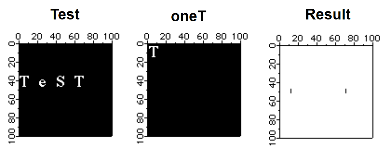
The FFT can be used to locate objects of a particular size and shape in a given image. The following example is rather simple in that the test object has the same scale and rotation angle as the ones found in the image.
// The test image contains the word Test.
NewImage test								// We will be looking for the two T's
Duplicate/O root:images:oneT oneT		// the object we are looking for
NewImage oneT

Duplicate/O test testf					// because the FFT overwrites
FFT testf
Duplicate/O oneT oneTf
FFT oneTf
testf*=oneTf							// not a "proper" correlation
IFFT testf
SetScale/P x 0,1,"", testf				// remove labels
SetScale/P y 0,1,"", testf
ImageThreshold/O/T=1.25e6 testf		// remove noise (due to overlap with other characters,
NewImage testf							// the results are the correlation spots for the T's)
When using the FFT it is sometimes necessary to operate on the source image with one of the built-in window functions so that pixel values go smoothly to zero as you approach image boundaries. The ImageWindow operation supports the Hanning, Hamming, Bartlett, Blackman, and Kaiser windows. Normally the ImageWindow operation works directly on an image as in the following example:
// The redimension is required for the FFT operation anyway, so you might
// as well perform it here and reduce the quantization of the results in
// the ImageWindow operation.
Redimension/s blobs
ImageWindow /p=0.03 kaiser blobs
NewImage M_WindowedImage
To see what the window function looks like:
Redimension/S blobs                     // SP or DP waves are necessary
ImageWindow/i/p=0.01 kaiser blobs       // just creates the window data
NewImage M_WindowedImage                // you can also make a surface plot from this.
Wavelet Transform
The wavelet transform is used primarily for smoothing, noise reduction and lossy compression. In all cases the procedure we follow is first to transform the image, then perform some operation on the transformed wave and finally calculate the inverse transform.
The next example illustrates a wavelet compression procedure. Start by calculating the wavelet transform of the image. Your choice of wavelet and coefficients can significantly affect compression quality. The compressed image is the part of the wave that corresponds to the low order coefficients in the transform (similar to low pass filtering in 2D Fourier transform). In this example we use the ImageInterpolate operation to create a wave from a 64x64 portion of the transform.
DWT /N=4/P=1/T=1 root:images:MRI,wvl_MRI            // perform the Wavelet transform
ImageInterpolate/S={0,1,63,0,1,63} bilinear wvl_MRI // reduce size by a factor of 16
To reconstruct the image and evaluate compression quality, inverse-transform the compressed image and display the result:
DWT /I/N=4/P=0/T=1 M_InterpolatedImage,iwvl_compressed
NewImage iwvl_compressed

The reconstructed image exhibits a number of compression-related artifacts, but it is worth noting that unlike an FFT based low-pass filter, the advantage of the wavelet transform is that the image contains a fair amount of high spatial frequency content. The factor of 16 mentioned above is not entirely accurate because the original image was stored as a one byte per pixel while the compressed image consists of floating point values (so the true compression ratio is only 4).
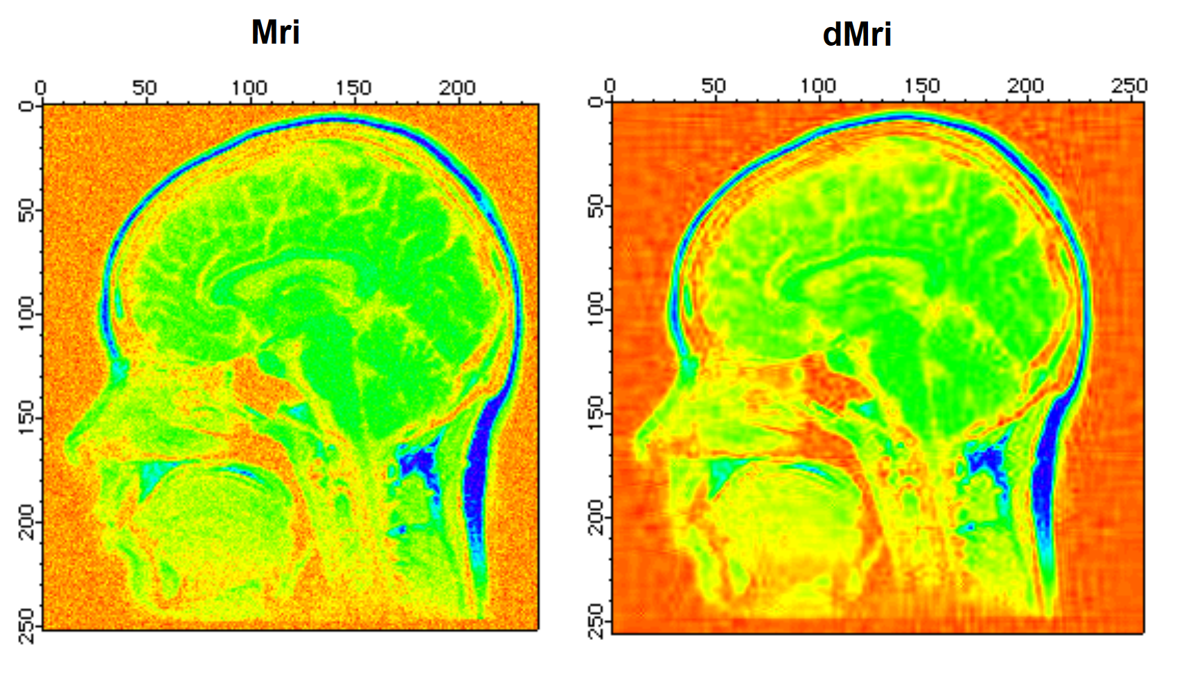
To illustrate the application of the wavelet transform to denoising, we start by adding Gaussian distributed noise with standard deviation 10 to the MRI image:
Redimension/S Mri                       // SP so we can add bipolar noise
Mri+=gnoise(10)                         // Gaussian noise added
NewImage Mri
ModifyImage Mri ctab={*,*,Rainbow,0}    // false color for better discrimination.
DWT/D/N=20/P=1/T=1/V=0.5 Mri,dMri       // increase /V for more denoising
NewImage dMri                           // display denoised image
ModifyImage dMri ctab={*,*,Rainbow,0}
Hough Transform
The Hough Transform is a mapping algorithm in which lines in image space map to single points in the transform space. It is most often used for line detection. Specifically, each point in the image space maps to a sinusoidal curve in the transform space. If pixels in the image lie along a line, the sinusoidal curves associated with these pixels all intersect at a single point in the transform space. By counting the number of sinusoids intersecting at each point in the transform space, lines can be detected. Here is an example of an image that consists of one line.
Make/O/B/U/N=(100,100) lineImage
lineImage=(p==q ? 255:0)			// single line at 45 degrees
Newimage lineimage
Imagetransform hough lineImage
Newimage M_Hough
The Hough transform of a family of lines:
lineImage=((p==100-q)|(p==q)|(p==50)|(q==50)) ? 255:0
Imagetransform Hough lineImage
The last image shows a series of bright pixels in the center. The first and last points correspond to lines at 0 and 180 degrees. The second point from the top corresponds to the line at 45 degrees and so on.

Fast Hartley Transform
The Hartley transform is similar to the Fourier transform except that it uses only real values. The transform is based on the cas kernel defined by:
The discrete Hartley transform is given by
The Hartley transform has two interesting mathematical properties. First, the inverse transform is identical to the forward transform, and second, the power spectrum is given by the expression:
The implementation of the Fast Hartley Transform is part of the ImageTransform operation. It requires that the source wave is an image whose dimensions are a power of 2.
ImageTransform /N={18,3}/O padImage Mri		// make the image 256^2
ImageTransform fht mri
NewImage M_Hartley
Convolution Filters
Convolution operators usually refer to a class of 2D kernels that are convolved with an image to produce a desirable effect (simple linear filtering). In some cases it is more efficient to perform convolutions using the FFT (similar to the convolution example above), i.e., transform both the image and the filter waves, multiply the transforms in the frequency domain and then compute the inverse transformation using the IFFT. The FFT approach is more efficient for convolution with kernels that are greater than 13x13 pixels. However, there is a very large number of useful kernels which play an important role in image processing that are 3x3 or 5x5 in size . Because these kernels are so small, it is fairly efficient to implement the corresponding linear filter as direct convolution without using the FFT.
In the following example we implement a low-pass filter with equal spatial frequency response along both axes.
Make /O/N=(9,9) sKernel						// first create the convolution kernel
SetScale/I x -4.5,4.5,"", sKernel
SetScale/I y -4.5,4.5,"", sKernel

// equivalent to rect(2*fx)*rect(2*fy) in the spatial frequency domain.
sKernel=sinc(x/2)*sinc(y/2)

// remember: MatrixConvolve executes in place; save your image first!
Duplicate/O root:images:MRI mri
Redimension/S mri							// to avoid integer truncation
MatrixConvolve sKernel mri
NewImage mri
ModifyImage mri ctab= {*,*,Rainbow,0}		// just to see it better
The next example illustrates how to perform edge detection using a built-in convolution filter in the ImageFilter operation:
Duplicate/O root:images:blobs blobs
ImageFilter findEdges blobs
NewImage blobs
Other notable examples of image filters are Gauss, Median and Sharpen. You can also apply the same operation to 3D waves. The filters Gauss3D, avg3D, point3D, min3D, max3D and median3Dare the extensions of their 2D counterparts to 3x3x3 voxel neighborhoods. Note that the last three filters are not true convolution filters.
Edge Detectors
In many applications it is necessary to detect edges/boundaries of objects that appear in images. The edge detection consists of creating a binary image from a grayscale image where the pixels in the binary image are turned off or on depending on whether they belong to region boundaries or not. In other words, the detected edges are described by an image, not a vector (1D wave). If you need to obtain a wave describing boundaries of regions, you might want to use the ImageAnalyzeParticles operation.
Igor supports eight built-in edge detectors (methods) that vary in performance depending on the source image. Some methods require that you provide several parameters which tend to have a significant effect on the quality of the result. In the following examples we illustrate the importance of these choices.
// create and display a simple artificial edge image
Make/B/U/N=(100,100) edgeImage
edgeImage=(p<50? 50:5)
Newimage edgeImage

// now try simple Sobel detector using iterated threshold detection
ImageEdgeDetection/M=1/N Sobel, edgeImage
NewImage M_ImageEdges
ModifyImage M_ImageEdges explicit=0		// to see this binary image in color
ModifyImage M_ImageEdges ctab= {*,*,Rainbow,0}
This result (the red line) is pretty much what we would expect. Here are other examples that work similarly well:
ImageEdgeDetection/M=1/N Kirsch, edgeImage // same output wave
or
ImageEdgeDetection/M=1/N Roberts, edgeImage // same output wave
The innocent looking /M=1 flag implies that the operation uses an iterative automatic thresholding. This appears to work well in the examples above, but it fails completely when using the Frei filter:
ImageEdgeDetection/M=1/N Frei, edgeImage
On the other hand, the bimodal fit thresholding works much better here:
ImageEdgeDetection/M=2/N Frei, root:edgeImage
Some of the more exotic edge detectors work best in the presence of noise and some variation of the grayscale. In the case of our simple image, they can miss the edge completely:
ImageEdgeDetection/M=1/N/S=1 Canny, edgeImage
The performance of this filter improves dramatically if you add a little noise to the image:
edgeImage+=gnoise(1)
ImageEdgeDetection/M=1/N/S=1 Canny, edgeImage
Using the More Exotic Edge Detectors
The more exotic edge detectors consist of multistep operations that usually involve smoothing and differentiation. Here is an example that illustrates the effect of smoothing:
Duplicate/O root:images:blobs blobs
ImageEdgeDetection/M=1/N/S=1 Canny,blobs
Duplicate/O M_ImageEdges smooth1
ImageEdgeDetection/M=1/N/S=2 Canny,blobs
Duplicate/O M_ImageEdges smooth2
ImageEdgeDetection/M=1/N/S=3 Canny,blobs
Duplicate/O M_ImageEdges smooth3
NewImage smooth1
ModifyImage smooth1 explicit=0
NewImage smooth2
ModifyImage smooth2 explicit=0
NewImage smooth3
ModifyImage smooth3 explicit=0
As you can see, the third image (smooth3) is indeed much cleaner than the first or the second, however, that result is obtained at the cost of loosing some of the small blobs. For example, execute the following to identify one of the missing blobs:
DoWindow/F Graph0
SetDrawLayer UserFront
SetDrawEnv linefgc= (65280,0,0),fillpat= 0
DrawOval 0.29,0.41,0.35,0.48
DoWindow/F Graph1
SetDrawLayer UserFront
SetDrawEnv linefgc= (65280,0,0),fillpat= 0
DrawOval 0.29,0.41,0.35,0.48
DoWindow/F Graph2
SetDrawLayer UserFront
SetDrawEnv linefgc= (65280,0,0),fillpat= 0
DrawOval 0.29,0.41,0.35,0.48
It is instructive to make a similar set of images using the Marr and Shen detectors.
// Note: This will take considerably longer to execute!
Duplicate/O root:images:blobs blobs
ImageEdgeDetection/M=1/N/S=1 Marr,blobs
Duplicate/O M_ImageEdges smooth1
ImageEdgeDetection/M=1/N/S=2 Marr,blobs
Duplicate/O M_ImageEdges smooth2
ImageEdgeDetection/M=1/N/S=3 Marr,blobs
Duplicate/O M_ImageEdges smooth3
NewImage smooth1
ModifyImage smooth1 explicit=0
NewImage smooth2
ModifyImage smooth2 explicit=0
NewImage smooth3
ModifyImage smooth3 explicit=0
SetDrawLayer UserFront
SetDrawEnv linefgc= (65280,0,0),fillpat= 0
DrawOval 0.29,0.41,0.35,0.48
The three images of the calculated edges demonstrate the reduction of noise with the increase in the size of the convolution kernel. It's also worth noting that the blob that disappeared when we used the Canny detector is clearly visible using the Marr detector.
In the following example we use the Shen-Castan detector with various smoothing factors. Note that this edge detection algorithm does not use the standard thresholding (you have to specify the threshold using the /F flag).
Duplicate/O root:images:blobs blobs
ImageEdgeDetection/N/S=0.5 shen,blobs
Duplicate/O M_ImageEdges smooth1
ImageEdgeDetection/N/S=0.75 shen,blobs
Duplicate/O M_ImageEdges smooth2
ImageEdgeDetection/N/S=0.95 shen,blobs
Duplicate/O M_ImageEdges smooth3
NewImage smooth1
ModifyImage smooth1 explicit=0
NewImage smooth2
ModifyImage smooth2 explicit=0
NewImage smooth3
ModifyImage smooth3 explicit=0
SetDrawLayer UserFront
SetDrawEnv linefgc=(65280,0,0),fillpat=0
DrawOval 0.29,0.41,0.35,0.48
As you can see in this example, the Shen detector produces a thin, though sometimes broken, boundary. The noise reduction is a tradeoff with edge quality.
One of the problems of edge detectors that employ smoothing is that they usually introduce errors when there are two edges that are relatively close to each other. In the following example we construct an artificial image that illustrates this point:
Make/B/U/O/N=(100,100) sampleEdge=0
sampleEdge[][49]=255
sampleEdge[][51]=255
NewImage sampleEdge
ImageEdgeDetection/N/S=1 Marr, sampleEdge
Duplicate/O M_ImageEdges s2
NewImage s2
ImageEdgeDetection/M=1/S=3 Canny, sampleEdge
Duplicate/O M_ImageEdges s3
NewImage s3

Note that the Marr detector completely misses the edge with the smoothing setting set to 1. Also, the position of the edge moves away from the true edge with increased smoothing in the Canny detector.
Morphological Operations
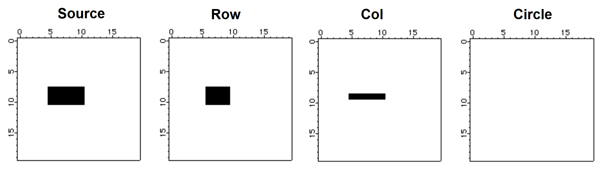
Morphological operators are tools that affect the shape and boundaries of regions in the image. Starting with dilation and erosion, the typical morphological operation involves an image and a structure element. The structure element is normally much smaller in size than the image. Dilation consists of reflecting the structure element about its origin and using it in a manner similar to a convolution mask. This can be seen in the next example:
Make/B/U/N=(20,20) source=0
source[5,10][8,10]=255                      // source is a filled rectangle
NewImage source
Imagemorphology /E=2 BinaryDilation source  // dilation with 1x3 structure element
Duplicate M_ImageMorph row
NewImage row                                // display the result of dialation
Imagemorphology /E=3 BinaryDilation source  // perform dilation by 3x1 column
Duplicate M_ImageMorph col
NewImage col                                // display column dilation
Imagemorphology /E=5 BinaryDilation source  // dilation by a circle
NewImage M_ImageMorph                       // display circle dilation

The result of erosion is the set of pixels x, y such that when the structure element is translated by that amount it is still contained within the set.
Make/B/U/N=(20,20) source=0
source[5,10][8,10]=255						// source is a filled rectangle
NewImage source
Imagemorphology /E=2 BinaryErosion source	// erosion with 1x3 structure element
Duplicate M_ImageMorph row
NewImage row									// display the result of erosion
Imagemorphology /E=3 BinaryErosion source	// perform erosion by 3x1 column
Duplicate M_ImageMorph col
NewImage col									// display column erosion
Imagemorphology /E=5 BinaryErosion source	// erosion by a circle
NewImage M_ImageMorph						// display circle erosion
We note first that the erosion by a circle erased all source pixels. We get this result because the circle structure element is a 5x5 "circle" and there is no x, y offset such that the circle is completely inside the source. The row and the col images show erosion predominantly in one direction. Again, try to imagine the 1x3 structure element (in the case of the row) sliding over the source pixels to produce the erosion.
The next pair of morphological operations are the opening and closing. Functionally, opening corresponds to an erosion of the source image by some structure element (say E), and then dilating the result using the same structure element E again. In general opening has a smoothing effect that eliminates small (narrow) protrusions as we show in the example below:
Make/B/U/N=(20,20) source=0
source[5,12][5,14] = 255
source[6,11][13,14] = 0
source[5,8][10,10] = 0
source[10,12][10,10] = 0
source[7,10][5,5] = 0
NewImage source
ImageMorphology /E=1 opening source	// opening using 2x2 structure element
Duplicate M_ImageMorph OpenE1
NewImage OpenE1
ImageMorphology /E=4 opening source	// opening using a 3x3 structure element
NewImage M_ImageMorph

As you can see, the 2x2 structure element removed the thin connection between the top and the bottom regions as well as the two protrusions at the bottom. On the other hand, the two protrusions at the top were large enough to survive the 2x2 structure element. The third image shows the result of the 3x3 structure element which was large enough to eliminate all the protrusions but also the bottom region as well.
The closing operation corresponds to a dilation of the source image followed by an erosion using the same structure element.
Make/B/U/N=(20,20) source=0
source[5,12][5,14] = 255
source[6,11][13,14] = 0
source[5,8][10,10] = 0
source[10,12][10,10] = 0
source[7,10][5,5] = 0
NewImage source
ImageMorphology /E=4 closing source	// closing using 3x3 structure element
Duplicate M_ImageMorph CloseE4
NewImage CloseE4
ImageMorphology /E=5 closing source	// closing using a 5x5 structure element
NewImage M_ImageMorph
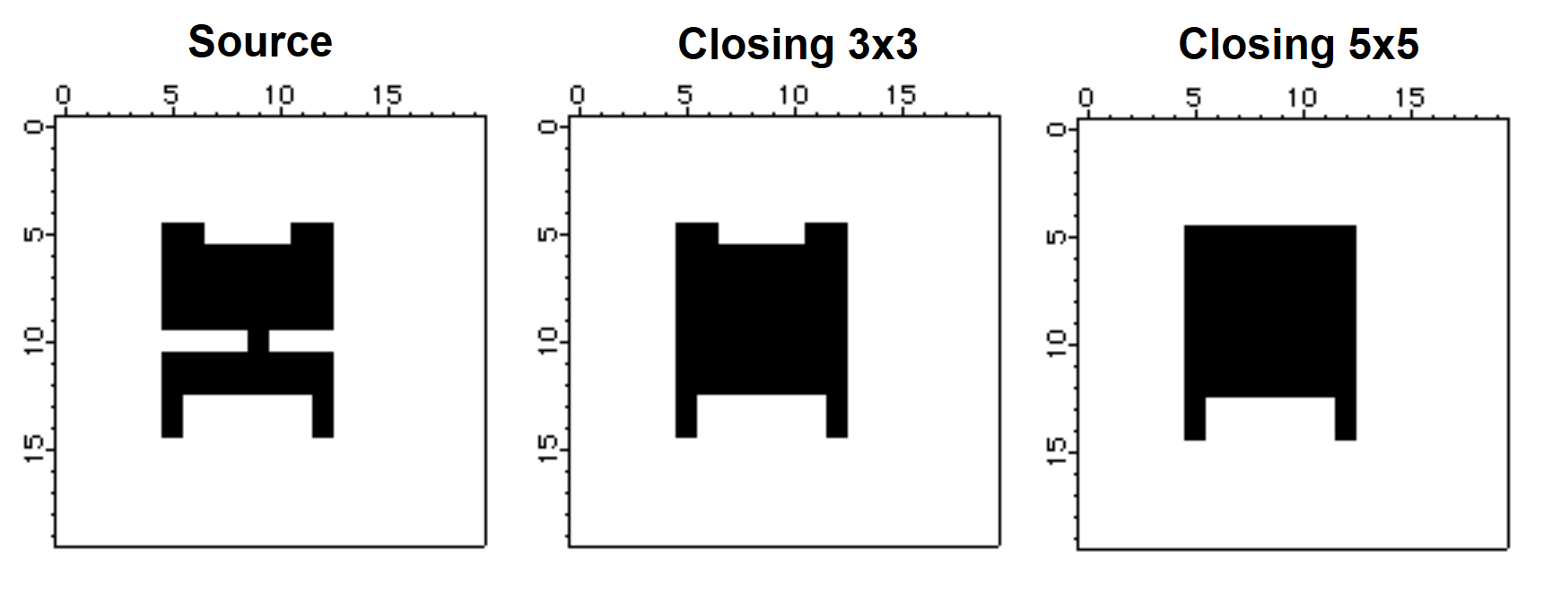
The center image above corresponds to a closing using a 3x3 structure element which appears to be large enough to close the gap between the top and bottom regions but not sufficiently large to fill the gaps between the top and bottom protrusions. The image on the right was created with a 5x5 "circle" structure element, which was evidently large enough to close the gap between the protrusions at the top but not at the bottom.
There are various interpretations for the Top Hat morphological operation. Igor's Top Hat calculates the difference between an eroded image and a dilated image. Other interpretations include calculating the difference between the image itself and its closing or opening. In the following example we illustrate some of these variations.
Duplicate root:images:mri source
ImageMorphology /E=1 tophat source	// closing using 2x2 structure element
Duplicate M_ImageMorph tophat
NewImage tophat
ImageMorphology /E=1 closing source	// closing using a 3x3 structure element
Duplicate M_ImageMorph closing
closing-=source
NewImage closing
ImageMorphology /E=1 opening source	// closing using a 3x3 structure element
Duplicate M_ImageMorph opening
opening=source-opening
NewImage opening

As you can see from the four images, the built-in Top Hat implementation enhances the boundaries (contours) of regions in the image whereas the opening or closing tophats enhance small grayscale variations.
The watershed operation locates the boundaries of watershed regions as we show below:
Make/O/N=(100,100) sample
sample=sinc(sqrt((x-50)^2+(y-50)^2)/2.5)	// looks like concentric circles.
ImageTransform/O convert2Gray sample
NewImage sample
ModifyImage sample ctab= {*,*,Terrain,0}	// add color for better discrimination
ImageMorphology /N/L watershed sample
AppendImage M_ImageMorph
ModifyImage M_ImageMorph explicit=1, eval={0,65000,0,0}

Note that omitting the /L flag in the watershed operation may result in spurious watershed lines as the algorithm follows 4-connectivity instead of 8.
Image Analysis
The distinction between image processing and image analysis is rather fine. The pure analysis operations are: ImageStats, line profile, histogram, hsl segmentation and particle analysis.
ImageStats Operation
You can obtain global statistics on a wave using the standard WaveStats operation. The ImageStats operation works specifically with 2D and 3D waves. The operation allows you to define a completely arbitrary ROI using a standard ROI wave (see Working with ROI). A special flag /M=1, allows you to speed up the operation when you only want to know the minimum, maximum and average values in the ROI region, skipping over the additional computation time required to evaluate higher moments. This operation was designed to work in user defined adaptive algorithms.
ImageStats can also operate on a specific plane of a 3D wave using the /P flag.
ImageLineProfile Operation
The ImageLineProfile operation is somewhat of a misnomer as it samples the image along a path consisting of an arbitrary number of line segments. To use the operation you first need to create the description of the path using a pair of waves. Here are some examples:
NewImage root:images:baboon					// Display the image that we want to profile
// create the pair of waves representing a straight line path
Make/O/N=2 xPoints={21,57}, yPoints={40,40}
AppendToGraph/T yPoints vs xPoints			// Display the path on the image

// calculate the profile
ImageLineProfile xwave=xPoints, ywave=yPoints, srcwave=root:images:baboon
Display W_ImageLineProfile vs W_LineProfileX	// Display the profile


You can create a more complex path consisting of an arbitrary number of points. In this case you may want to take advantage of the W_LineProfileX and W_LineProfileY waves that the operation creates and plot the profile as a 3D path plot (see Path Plots). See also the IP Tutorial experiment for more elaborate examples.
If you are working with 3D waves with more than 3 layers, you can use ImageLineProfile/P=plane to specify the plane for which the profile is computed.
If you are using the line profile to extract a sequential array of data (a row or column) from the wave it is more efficient (about a factor of 3.5 in speed) to extract the data using ImageTransform getRow or getCol.
Histograms
The histogram is a very important tool in image analysis. For example, the simplest approach to automating the detection of the background in an image is to calculate the histogram and to choose the pixel value which occurs with the highest frequency. Histograms are also very important in determining threshold values and in enhancing image contrast. Here are some examples using image histograms:
NewImage root:images:mri
ImageHistogram root:images:mri
Duplicate W_ImageHist origMriHist
Display /W=(201.6,45.2,411,223.4) origMriHist

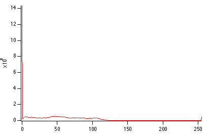
It is obvious from the histogram that the image is rather dark and that the background is most likely zero. The small counts for pixels above 125 suggests that the image is a good candidate for histogram equalization.
ImageHistModification root:images:mri
ImageHistogram M_ImageHistEq
NewImage M_ImageHistEq
AutoPositionWindow/E/M=1 /R=Graph0 $WinName(0,1)
Display /W=(201.6,45.2,411,223.4) W_ImageHist

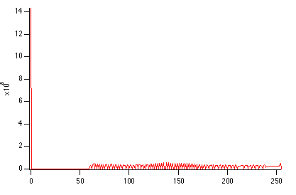
Comparing the two histograms we can see two immediate features: first, there is no change in the dark background because it is only one level (0). Second, the rest of the image which was mostly between the values of 0 and 120 has now been stretched to the range 57-255.
The next example illustrates how you can use the histogram information to determine a threshold value.
NewImage root:images:blobs
ImageHistogram root:images:blobs
Display /W=(201.6,45.2,411,223.4) W_ImageHist
The resulting histogram is clearly bimodal. Just for the fun of it, lets fit it to a pair of Gaussians:
// guess coefficient wave based on the histogram
Make/O/N=6 coeff={0,3000,50,10,500,210,20}
Funcfit/Q twoGaussians,coeff,W_ImageHist /D
ModifyGraph rgb(fit_W_ImageHist)=(0,0,65000)

The curve shown in the graph is the functional fit of the sum of two Gaussians. You can now choose, by visual inspection, an x-value between the two Gaussians -- probably somewhere in the range of 100-150. In fact, if you test the same image using the built-in thresholding operations that we have discussed above, you will see that the iterated algorithm chooses the value 125, fuzzy entropy chooses 109, etc.
Histograms of RGB or HSL images result in a separate histogram for each color channel:
ImageHistogram root:images:peppers
Display W_ImageHistR,W_ImageHistG,W_ImageHistB
ModifyGraph rgb(W_ImageHistG)=(0,65000,0),rgb(W_ImageHistB)=(0,0,65000)

Histograms of 3D waves containing more than 3 layers can be computed by specifying the layer with the /P flag. For example,
Make/N=(10,20,30) ddd=gnoise(5)
ImageHistogram/P=10 ddd
Display W_ImageHist
Unwrapping Phase
Unwrapping phase in two dimensions is more complicated than in one dimension because the operation's results must be independent of the unwrapping path. The path independence means that any path integral over a closed contour in the unwrapped domain must vanish. In many situations there are points in the domain around which closed contour path integrals do not vanish. Such points are called "residues". The residues are positive if a counter-clockwise path integral is positive. When unwrapping phase in two dimensions, the residues are typically ±1. This suggests that whenever two opposing residues are connected by a line (known as a "branch cut"), any contour integral whose path does not cross the branch cut will vanish. When a positive and negative residues are side by side they combine to a "dipole" which may be removed because a path integral around the dipole also vanishes. It follows that unwrapping can be performed using paths that either do not encircle unbalanced residues or paths that do not cross branch cuts.
The ImageUnwrapPhase operation performs 2D phase unwrapping using either a fast method that ignores possible residues or a slower method which locates residues and attempts to find paths around them. The fast method uses direct integration of the differential phases. It can lead to incorrect results if there are residues in the domain. The slow method first identifies all residues, draws them into an internal bitmap adding branch cuts and then applying repeatedly the algorithm used in ImageSeedFill to obtain the paths around the residues and branch cuts until all pixels have been processed. Sometimes the distribution of residues and branch cuts is such that the domain of the data is covered by several regions, each of which is completely bounded by branch cuts or the data boundary. In this case, the phase is computed independently in each individual region with an offset that is based on the first processed pixel in that region. Note that when you use ImageUnwrapPhase using a method that computes the residues, the operation creates the variables V_numResidues and V_numRegions. You can also obtain a copy of the internal bitmap which could be useful for analyzing the results.
The ImageUnwrapPhase Demo in the Examples:Analysis folder provides a detailed example illustrating different types of residues, branch cuts and resulting unwrapped phase.
Image Registration Demo
HSL Segmentation
When you work with color images you have two analogs to grayscale thresholding. The first is simple thresholding of the luminance of the image. To do this you need to convert the image from RGB to HSL and then perform the thresholding on the luminance plane. The second equivalent of thresholding is HSL segmentation, where the image is subdivided into regions of HSL values that fall within a certain range. In the following example we segment the peppers image to locate regions corresponding to red peppers:
NewImage root:images:peppers
ImageTransform/H={330,50}/L={0,255}/S={0,255} root:images:peppers
NewImage M_HueSegment
Note that we have used /H={330,50}. The apparent flip of the limits is allowed in the case of hue values in order to cover the single range from hue angle 330 degrees to hue angle 50 degrees.
Particle Analysis
Typical particle analysis consists of three steps. First you need to preprocess the image. This may include noise removal/reduction, possible background adjustments (see ImageRemoveBackground) and thresholding. Once you obtain a binary image, your second step is to invoke the ImageAnalyzeParticles operation. The third and final step is making some sense of all the data produced by the ImageAnalyzeParticles operation or "post-processing".
Issues related to the preprocessing have been discussed elsewhere in this help file. We will assume that we are starting with a preprocessed, clean, binary image which contains some particles.
NewImage root:images:blobs					// display the original image

// Step 1: create binary image.
// Note the /I flag to invert the output wave so that particles are marked by zero.
ImageThreshold/I/Q/M=1 root:images:blobs	// Note the /I flag!!!

// Step 2: Here we are invoking the operation in quiet mode,
// specifying particles of size equal or greater than 2 pixels. We are also
// asking for particles moment information, boundary waves and a
// particle masking wave.
ImageAnalyzeParticles /Q/A=2/E/W/M=2 stats M_ImageThresh

// Step 3: post processing choices
// Display the detected boundaries on top of the particles
AppendToGraph/T W_BoundaryY vs W_BoundaryX

// If you browse the numerical data:
Edit W_SpotX,W_SpotY,W_circularity,W_rectangularity,W_ImageObjPerimeter
AppendToTable W_xmin,W_xmax,W_ymin,W_ymax,M_Moments,M_RawMoments
Particles that intersect the boundary of the image may give rise to inaccuracies in particle statistics. It is therefore useful sometimes to remove these particles before performing the analysis.
The raw values generated by ImageAnalyzeParticles operation can be used for further processing.
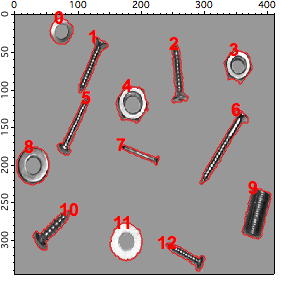
The following example illustrates slightly different pre and post-processing.
NewImage screws
// here we have a synthetic background so the conversion to binary is easy.
screws=screws==163 ? 255:0
ImageMorphology /O/I=2/E=1 binarydilation screws
ImageMorphology /O/I=2/E=1 erosion screws

// Now the particle analysis operation with the option to fill the holes
ImageAnalyzeParticles/E/W/Q/M=3/A=5/F stats, screws

NewImage root:images:screws
AutoPositionWindow/E $WinName(0,1)
// show the detected boundaries
AppendToGraph/T W_BoundaryY vs W_BoundaryX
AppendToGraph/T W_SpotY vs W_SpotX
Duplicate/O w_spotx w_index
w_index=p
ModifyGraph mode(W_SpotY)=3
ModifyGraph textMarker(W_SpotY)={w_index,"default",1,0,5,0.00,0.00}
ModifyGraph msize(W_SpotY)=6
// Now for some shape classification: plot particle area vs perimeter
Display/W=(23.4,299.6,297,511.4) W_ImageObjArea vs W_ImageObjPerimeter
ModifyGraph mode=3,textMarker(W_ImageObjArea)={w_index,"default",0,0,5,0.00,0.00}
ModifyGraph msize=6

The classification diagram we just created uses two parameters (area and perimeter) that are very sensitive to image noise. We can see that there are two basic classes that can be associated with the roundness of the boundaries but it is difficult to accept the classification of particle 9.
In the following we compute another classification based on the eccentricity of the objects:
Make/O/N=(DimSize(M_Moments,0)) ecc
ecc=sqrt(1-M_Moments[p][3]^2/M_Moments[p][2]^2)

Display /W=(23.4,299.6,297,511.4) ecc
ModifyGraph mode=3,textMarker(ecc)={w_index,"default",0,0,5,0.00,0.00}
ModifyGraph msize=6

The second classification provides a perfect distinction between the screws and the washers/nuts. It also illustrates the importance of selecting the best classification parameters.
You can use the ImageAnalyzeParticles operation also for the purpose of creating masks for particular particles. For example, to create a mask for particle 9 in the example above:
ImageAnalyzeParticles /L=(w_spotX[9],w_spotY[9]) mark screws
NewImage M_ParticleMarker
You can use this feature of the operation to color different classes of objects using an overlay.
Seed Fill
In some situations you may need to define segments of the image based on a contiguous region of pixels whose values fall within a certain range. The ImageSeedFill operation helps you do just that.
NewImage mri
ImageSeedFill/B=64 seedX=132,seedY=77,min=52,max=65,target=255,srcWave=mri
AppendImage M_SeedFill
ModifyImage M_SeedFill explicit=1, eval={255,65535,65535,65535}

Here we have used the /B flag to create an overlay image but it can also be used to create an ROI wave for use in further processing. This example represents the simplest use of the operation. In some situations the criteria for a pixel's inclusion in the filled region are not so sharp and the operation may work better if you use the adaptive or fuzzy algorithms. For example:
ImageSeedFill/B=64/c seedX=144,seedY=83,min=60,max=150, target=255,srcWave=mri,adaptive=3
Note that the min and max values have been relaxed but the adaptive parameter provides alternative continuity criterion.
Other Tools
Igor provides a number of utility operations to help you manage and manipulate image data.
Working with ROI
Many of the image processing operations support a region of interest (ROI). The region of interest is the portion of the image that we want to affect by an operation. Igor supports a completely general ROI, specified as a binary wave (unsigned byte) that has the same dimensions as the image. Set the ROI wave to zero for all pixels within the region of interest and to any other value outside the region of interest. Note that in some situations it is useful to set the ROI pixels to a nonzero value (e.g., if you use the wave as a multiplicative factor in a mathematical operation). You can use ImageTransform with the keyword "invert" to quickly convert between the two options.
The easiest way to create an ROI wave is directly from the command line. For example, an ROI wave that covers a quarter of the blobs image may be generated as follows:
Duplicate root:images:blobs myROI
Redimension/B/U myROI
myROI=64                        // arbitrary nonzero value
myROI[0,128][0,127]=0           // the actual region of interest

// Example of usage:
ImageThreshold/Q/M=1/R=myROI root:images:blobs
NewImage M_ImageThresh

If you want to define the ROI using graphical drawing tools you need to open the tools and set the drawing layer to progFront. This can be done with the following instructions:
SetDrawLayer progFront
ShowTools/A rect		// selects the rectangle drawing tool first
Generating ROI Masks
You can now define the ROI as the area inside all the closed shapes that you draw. When you complete drawing the ROI you need to execute the commands:
HideTools/A								// drawing tools are not needed any more.
ImageGenerateROIMask M_ImageThresh	// M_ImageThresh is the top image in this example.

// your ROI wave has been created; To see it,
NewImage M_ROIMask
The Image Processing procedures provide a utility for creating an ROI wave by drawing on a displayed image.
Converting Boundary to a Mask
A third way of generating an ROI mask is using the ImageBoundaryToMask operation. This operation takes a pair of waves (y versus x) that contain pixel values and scan-converts them into a mask. When you invoke the operation you also have to specify the rectangular width and height of the output mask.
// create a circle
Make/N=100 ddx,ddy
ddx=50*(1-sin(2*pi*x/100))
ddy=50*(1-cos(2*pi*x/100))
ImageBoundaryToMask width=100,height=100,xwave=ddx,ywave=ddy
// The result is an image not a curve!
NewImage M_ROIMask
Note that the resulting binary wave has the values 0 and 255 which you may need to invert before using in some operations.
In many situations the operation ImageBoundaryToMask is followed by ImageSeedFill in order to convert the mask to a filled region. You can obtain the desired mask in one step using the keywords seedX and seedY in ImageBoundaryToMask but you must make sure that the mask created by the boundary waves is a closed domain.
ImageBoundaryToMask width=100,height=100,xwave=ddx,ywave=ddy, seedX=50,seedY=50
ModifyImage M_ROIMask explicit=0
Marquee Procedures
A fourth way to create an ROI mask is using the Marquee2Mask procedures. To use this in your own experiment you will have to add the following line to your procedure window:
#include <Marquee2Mask>
You can now create the ROI mask by selecting one or more rectangular marquees (click and drag the mouse) in the image. After you select each marquee click inside the marquee and choose MarqueeToMask or AppendMarqueeToMask.
Subimage Selection
You can use an ROI to apply various image processing operations to selected portions of an image. The ROI is a very useful tool especially when the region of interest is either not contiguous or not rectangular. When the region of interest is rectangular, you can usually improve performance by creating a new subimage which consists entirely of the ROI. If you know the coordinates and dimensions of the ROI it is simplest to use the Duplicate/R operation. If you want to make an interactive selection you can use the marquee together with CopyImageSubset marquee procedure (after making a marquee selection in the image, click inside the marquee and choose CopyImageSubset).
Handling Color
Most of the image operations are designed to work on grayscale images. If you need to perform an operation on a color image certain aspects become a bit more complicated. In the example below we illustrate how you might sharpen a color image.
NewImage root:images:rose
ImageTransform rgb2hsl root:images:rose	// first convert to hsl
ImageTransform/P=2 getPlane M_RGB2HSL
ImageFilter Sharpen M_ImagePlane			// you can also use sharpenmore
ImageTransform /D=M_ImagePlane /P=2 setPlane M_RGB2HSL
ImageTransform hsl2rgb M_RGB2HSL
NewImage M_HSL2RGB
Background Removal
There are many approaches to removing the effect of a nonuniform background from an image. If the non uniformity is additive, it is sometimes useful to fit a polynomial to various points which you associate with the background and then subtract the resulting polynomial surface from the whole image. If the non uniformity is multiplicative, you need to generate an image corresponding to the polynomial surface and use it to scale the original image.
Additive Background
Duplicate/O root:images:blobs addBlobs
Redimension/S addBlobs			// convert to single precision
addBlobs+=0.01*x*y				// add a tilted plane
NewImage addBlobs
To use the ImageRemoveBackground operation, we need an ROI mask designating regions in the image that represent the background. You can create one using one of the ROI construction methods that we discussed above. For the purposes of this example, we choose the ROI that consists of the 7 rectangles shown in the Degraded Source image below.
// show us the ROI background selection
AppendImage root:images:addMask
ModifyImage addMask explicit=1, eval={1,65000,0,0}

// now create a corrected image and display it
ImageRemoveBackground /R=root:images:addMask /w/P=2 addBlobs
NewImage M_RemovedBackground

If the source image contains relatively small particles on a nonuniform background, you may remove the background (for the purpose of particle analysis) by iterating grayscale erosion until the particles are all gone. You are then left with a fairly good representation of the background that can be subtracted from the original image.
Multiplicative Background (Nonuniform Illumination)
This case is much more complicated because the removal of the background requires division of the image by the calculated background (it is assumed here that the system producing the image has an overall gamma of 1). The first complication has to do with the possible presence of zeros in the calculated background. The second complication is that the calculations give us the additional freedom to choose one constant factor to scale the resulting image. There are many approaches for correcting a multiplicative background. The following example shows how an image can be corrected if we assume that the peak values (identified by the ROI mask should have the same value in an ideal situation).
Duplicate/O root:images:blobs mulBlobs
Redimension/S mulBlobs	// convert to single precision
mulBlobs*=(1+0.005*x*y)
NewImage mulBlobs

// show us the ROI foreground selection;
// you can use histogram equalization to find fit regions in the dark area.
AppendImage root:images:multMask
ModifyImage multMask explicit=1, eval={1,65000,0,0}

ImageRemoveBackground /R=root:images:multMask/F/w/P=2 mulBlobs
// normalize the fit
WaveStats/Q/M=1 M_RemovedBackground

// renormalize the fit--we can use that one free factor.
M_RemovedBackground=(M_RemovedBackground-V_min)/(V_max-V_min)
// remove zeros by replacing with average value.
WaveStats/Q/M=1 M_RemovedBackground
MatrixOp/O M_RemovedBackground=M_RemovedBackground+V_avg*equal(M_RemovedBackground,0)
MatrixOp/O mulBlobs=mulBlobs/M_RemovedBackground		// scaled image.
In the example above we have manually created the ROI masks that were needed for the fit. You can automate this process (and actually improve performance) by subdividing the image into a number of smaller rectangles and selecting in each one the highest (or lowest) pixel values. An example of such procedure is provided in connection with the ImageStats operation above.
General Utilities: ImageTransform Operation
As we have seen above, the ImageTransform operation provides a number of image utilities. As a rule, if you are unable to find an appropriate image operation check the options available under ImageTransform. Here are some examples:
When working with RGB or HSL images it is frequently necessary to access one plane at a time. For example, the green plane of the peppers image can be obtained as follows:
NewImage root:images:peppers			// display original
Duplicate/O root:images:peppers peppers
ImageTransform /P=1 getPlane peppers
NewImage M_ImagePlane					// display green plane in grayscale
The complementary operation allows you to insert a plane into a 3D wave. For example, suppose you wanted to modify the green plane of the peppers image:
ImageHistModification/o M_ImagePlane
ImageTransform /p=1 /D=M_ImagePlane setPlane peppers
NewImage peppers						// display the processed image
Some operations are restricted to waves of particular dimensions. For example, if you want to use the Adaptive histogram equalization, the number of horizontal and vertical partitions is restricted by the requirement that the image be an exact multiple of the dimensions of the subregion. The ImageTransform operation provides three image padding options: If you specify a negative number to the changed rows or columns, the corresponding rows and columns are removed from the image. If the numbers are positive, rows and columns are added. By default the added rows and columns contain exactly the same pixel values as the last row and column in the image. If you specify the /W flag the operation duplicates the relevant portion of the image into the new rows and columns. Here are some examples:
Duplicate/o root:images:baboon baboon
NewImage baboon
ImageTransform/N={-20,-10} padImage baboon
Rename M_PaddedImage, cropped
NewImage cropped
ImageTransform/N={40,40} padImage baboon
Rename M_PaddedImage, padLastVals
NewImage padLastVals
ImageTransform/W/N={100,100} padImage baboon
NewImage M_PaddedImage
Another utility operation is the conversion of any 2D wave into a normalized (0-255) 8-bit image wave. This is accomplished with the ImageTransform operation using the keyword convert2gray. Here is an example:
// create some numerical data set
Make/O/N=(50,80) numericalWave=x*sin(x/10)*y*exp(y/100)
ImageTransform convert2gray numericalWave
NewImage M_Image2Gray
The conversion into 8-bit image is required for certain operation. It is also useful sometimes when you want to reduce the size of your image waves.
Image Processing References
Ghiglia, Dennis C., and Mark D. Pritt, Two Dimensional Phase Unwrapping -- Theory, Algorithms and Software, John Wiley & Sons, 1998.
Gonzalez, Rafael C., and Richard E. Woods, Digital Image Processing, 3rd ed., Addison-Wesley, 1992.
Pratt, William K., Digital Image Processing, 2nd ed., John Wiley & Sons, 1991.
Thévenaz, P., and M. Unser, A Pyramid Approach to Subpixel Registration Based on Intensity, IEEE Transactions on Image Processing, 7, 27-41, 1998.